13 250: Working with genomic data in R with the DECIPHER package

Authors: Nicholas Cooley²⁴ Last Modified: 18 July, 2018

13.1 Overview

13.1.1 Workshop Description

In this workshop we will give an introduction to working with biological sequence data in R using the Biostrings and DECIPHER packages. We will cover:

Importing, viewing, and manipulating genomes in R
Construction of sequence databases for organizing genomes
Mapping syntenic regions between genomes with the FindSynteny function
Understanding, accessing, and viewing objects of class Synteny
Using syntenic information to predict orthologous genes
Alignment of sequences and genomes with DECIPHER
Downstream analyses enabled by syntenic mapping

13.1.2 Pre-requisites

Familiarity with Biostrings
Familiarity with DECIPHER Databases²⁵

13.1.3 Workshop Participation

This will be a lab where participants follow along on their computers.

13.1.4 R / Bioconductor packages used

Biostrings
DECIPHER
stringr
FindHomology

13.1.5 Time outline

Activity	Time
Packages/Introduction	5m
Basic commands for sequences	5m
Sequence databases	10m
Demonstration of synteny mapping	10m
Explanation of function arguments	10m
Dissecting Synteny objects	10m
Visualization of syntenic blocks	10m
Alignment of syntenic regions	10m
Ortholog prediction from Synteny	10m
Constructing phylogenetic trees	10m

13.2 Workshop goals and objectives

13.2.1 Learning goals

Understand a simple workflow for analysis of sequences in R and DECIPHER
Learn the basic use and appropriate application of functions within DECIPHER

13.2.2 Learning objectives

Learn basic commands for working with sequences in R
Import genomes from online repositories or local files
Map synteny between genomes
Analyze a synteny map among multiple genomes
Develop an understanding of the data structures involved
Predict orthologs from syntenic maps
Select core and pan genomes from predicted orthologs
Construct and interpret phylogenetic trees

13.2.2.1 Introduction

In this worshop we will be walking through a comparative genomics pipeline using functions within the R package DECIPHER, and within a package that is currently under construction under the name FindHomology.

13.2.2.2 Context

Lipid membranes are ubiquitious in living organisms, however the individual lipid molecules that compose membranes have a wide variety of structures. The biosynthesis of common lipid molecules is well understood, conversely the biosynthesis of more exotic lipid molecules is not. The genomes selected today are from the archaeal phylum Thaumarchaeota, which are known for being anammox archaea, and are important in the nitrogen cycle. In addition to that, these archaea all produce a series of unusual lipids. Since these lipids are shared across the entire phylum from which these genomes are pulled, it is possible that the biosynthetic genes responsible for lipid construction are shared across the selected genomes, and part of their ‘core’ genome.

Archaea are relatively newly characterized as organisms. First classified in the ’70s²⁶, for their deviations from Prokaryotes, many Archaea are noteable for being isolated from extreme environments. Despite the colorful beginnings of their classification, not all Archaea are extremophiles.

Figure 13.1: Grand Prismatic Spring in Yellowstone National Park (3)

The aforementioned unusual lipds²⁷ are striking in their differences from those common in both Eukaryotes and Prokaryotes.

Figure 13.2: A. A generic lipid with phosphatidyl serine head group B. A generic Archaeal lipid C. A more exotic Archaeal lipid

Whereas Lipid construction in eucharyotes and prokaryotes relies on iterative incorporation of malonyl-CoA units, archaea utilize the melvonate pathway to construct their lipids through iterative incorporation of dimethylallyl pyrophosphate. Which is responsible for the iterative methyl groups extant to the lipid chain in B above. Archaeal lipids are also notable for their lack of ester linkages between the alkyl chain, and glyerol. Even more interesting, and as yet uncharacterized, Archaea incorporate a range of ring structures into their lipids, and additionally appear to fuse lipid tails together in the bilayer, as shown above in C.

13.2.2.3 The above is interesting, but so what?

Our goal with this workshop is to show how functions within DECIPHER, in addition to those found within FindHomology can be used to predict homologs between genomes, as well as predict the core genome of a given set of genomes. As stated above, the chemistry and biology involved in some of the construction of archaeal lipids is unknown. Hypothetically, as this chemistry is universal in these organisms, the genes responsible could all be homologs, and be identified as part of the core genome. Further we can compare the core and pan genomes of this set.

To begin with, we will load the required packages: DECIPHER and FindHomology will provide tools to complete the phylogenetic analysis, while phytools will provide visualization tools, specifically for the visualization of tangelograms, and stringr is used for a specific string operation.

13.2.2.4 Packages and Sequences

suppressMessages(library(DECIPHER))
library(FindHomology)
library(stringr)

13.2.2.5 Genomes, and DECIPHER databases

The first step in this process is selecting the genomes we want to work with. There are several ways to do this, especially when accessing publically available genomes through the NCBI. Entrez Direct²⁸ provides powerful unix command line tools, if that’s your flavor, but the NCBI Genome List, and other search tools are easily accessible, and have a lower barrier to to entry.

For the purposes of this workshop, we will be using a set of preselected genomes that will be accessed via ftp addresses. These are loaded with the FindHomology Package and can be accessed easily.

data("GeneCallAdds")
data("GenomeAdds")
data("GenomeIDs")

We have now loaded in a character vector for ftp addresses for genomic fasta files GenomeAdds, a character vector of ftp addresses for genomic GFF files GeneCallAdds that we will be using to collect gene boundaries, strandedness, and annotations. And lastly a vector of abbreviated names for the genomes we are working with.

FindHomology contains a simple parser function for GFF files that allows us to grab gene boundaries and annotations.

GeneCalls <- FindHomology::GFFParser(GFFAddress = GeneCallAdds,
                                     Verbose = TRUE)
#> ===========================================================================
#> Time difference of 7.574508 secs

If you choose to mimic this work on your own, there are a few ways to get gene calls(the gene boundaries, and strandedness), and annotations, such as Prodigal²⁹ (for gene calls) and Prokka³⁰ (for annotations). Using the NCBI annotations is simple and conducive for this workshop. However if you are working on sequence data that you have generated or collected yourself, NCBI annotations will not be available. Additionally, a Gene Caller within the DECIPHER package is currently under construction.

13.2.2.6 DECIPHER and Databases

DECIPHER works with sequence data through SQL databases. There are several reasons for this.

Figure 13.3: Databases are compressable and easily shareable

Databases provide large improvements in file organization. Currently, a personalized analysis pipeline could include anywhere from one to tens of programs, all of which may take in similar data, or outputs of previous steps, or may output more files than a user needs. DECIPHER’s use of databases allows for sequence data to be stored in an organized format that eliminates this kind of redundancy.

Use of databases also allows for a non-destructive workflow. Sequence data in the database can be accessed as needed, but cannot be accidentally manipulated. Databases are also shareable, allowing for accession by multiple users at once.

Additionally, constructing a database in DECIPHER is relatively easy.

In your own work, it can be inadvisable to use tempfile() to specify the location of your .sqlite file, especially if it will be a file you use repeatedly, or takes a significant amount of time to create, or that you will eventually need to share with collaborators. However for this workhshop, it is fine.

We can access our databases through either a database connection, or simply a filepath to the database. In this code chunk below, we will use a database connection.


DBPath <- tempfile()

DBConn <- dbConnect(SQLite(),
                    DBPath)

for (i in seq_along(GenomeAdds)) {
  Seqs2DB(seqs = GenomeAdds[i],
          type = "FASTA",
          dbFile = DBConn,
          identifier = as.character(i),
          tblName = "Seqs",
          verbose = FALSE)
}

dbDisconnect(DBConn)

Identifying details of the database can be viewed in your default browser: BrowseDB(DBPath)

13.2.2.7 Comparison of genomes

Comparison of genomes will be accomplished with Synteny. Generically when regions in a genome are the same, they are syntenic matches. Often observing this phenomenon is accomplished through matching runs of reciprocal best blast hits. If in genome 1, genes A-B-C are reciprocal best blast hits to genes Z-Y-X in genome 2, the region encompassing those genes would be considered syntenic.

In DECIPHER this is accomplished using k-mer matching, runs of an exact match of length k are identified and recorded as a syntenic hit.

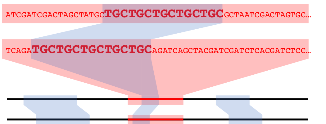
Figure 13.4: A syntenic hit in nucleotide space

We can visualize syntenic hits as above, with co-linear representations of genomes with some graphical links to signify the locations and lengths of syntenic hits. Or we can employ a dotplot, which utilizes the cumulative nucleotide positions of two genomes as the x and y axes in a generic plot.

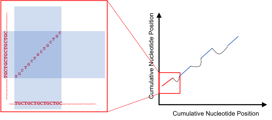
Figure 13.5: A syntenic hit, and several hits being chained toegher into a syntenic block

Syntenic Hits can be chained together, if they are close enough, to form larger syntenic blocks. The enough part, has to be measured in nucleotide distance between the hits in question, in both genomes. This also means that syntenic hits can be chained together with differing distances between them in each genome. Making syntenic blocks different lengths in corresponding genomes. Additionally, chaining of hits allows for utilizing smaller syntenic hits that may appear insignificant on their own, to be grouped in with other nearby hits to increase their significance.

DECIPHER’s FindSynteny function allows users to control the degree to which hits and blocks are recorded through the argument minScore, or a minimum score required for a block, or hit, to be kept as a real syntenic match.

In this workflow, we will be determining Synteny between genomes before we consider the gene calls we have already collected. Which stands in contrast to how many current synteny finding programs work. In the code below FindSyntey() will perform pairways analysis of every set of genomes provided to it.

# Here we will use a file path instead of a dbconnection
SyntenyObject <- FindSynteny(dbFile = DBPath,
                             verbose = TRUE)
#> ===========================================================================
#> 
#> Time difference of 58.81 secs

There are multiple ways to view objects of class synteny. It has default view options for plot(). By default, colors are assigned as a ramp from the first nucleotide position, to the last nucleotide position of the query genome, or the first genome selected, and wherever syntenic hits are observed, the bar representing the subject genome is marked with the section of the color ramp indicating the syntenic hit in the query.

Plotting genomes 2 and 3, which are very syntenic, provides a good example of this. Grey uncolored space in the subject genome indicates a lack of syntenic blocks in that region. In some places, the ramp reverses, indicating an inversion, while in others, blocks are reordered from the default color bar, indicating possible rearrangements.

plot(SyntenyObject[2:3, 2:3])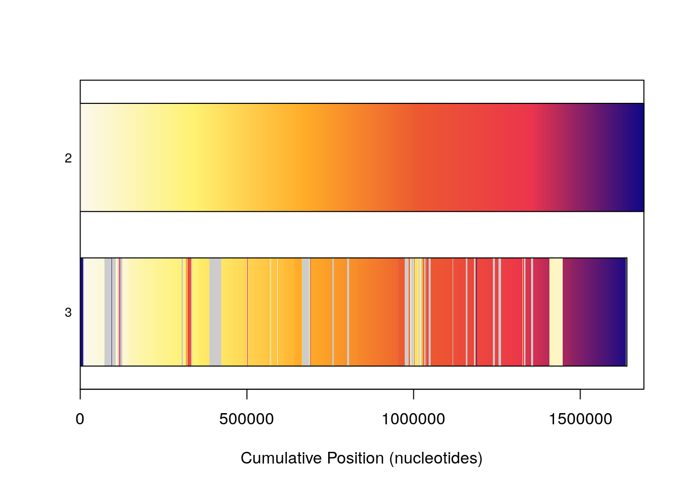

Because visualizing large numbers of syntenic hits in genome sized sequences can be non-trivial, additional commands can be passed to plot in order to modify coloring schemes. frequency causes bars representing genomes to be colored by how syntenic that particular region (as determined by cumulative nucleotide position) of the genome is, indiscriminate of where that hit is in a corresponding genome. Once again genomes 2 and 3 in our set are good examples of this. They are highly syntenic, which this option shows well, but the rearrangements present are no longer shown.

plot(SyntenyObject[2:3, 2:3],
     "frequency")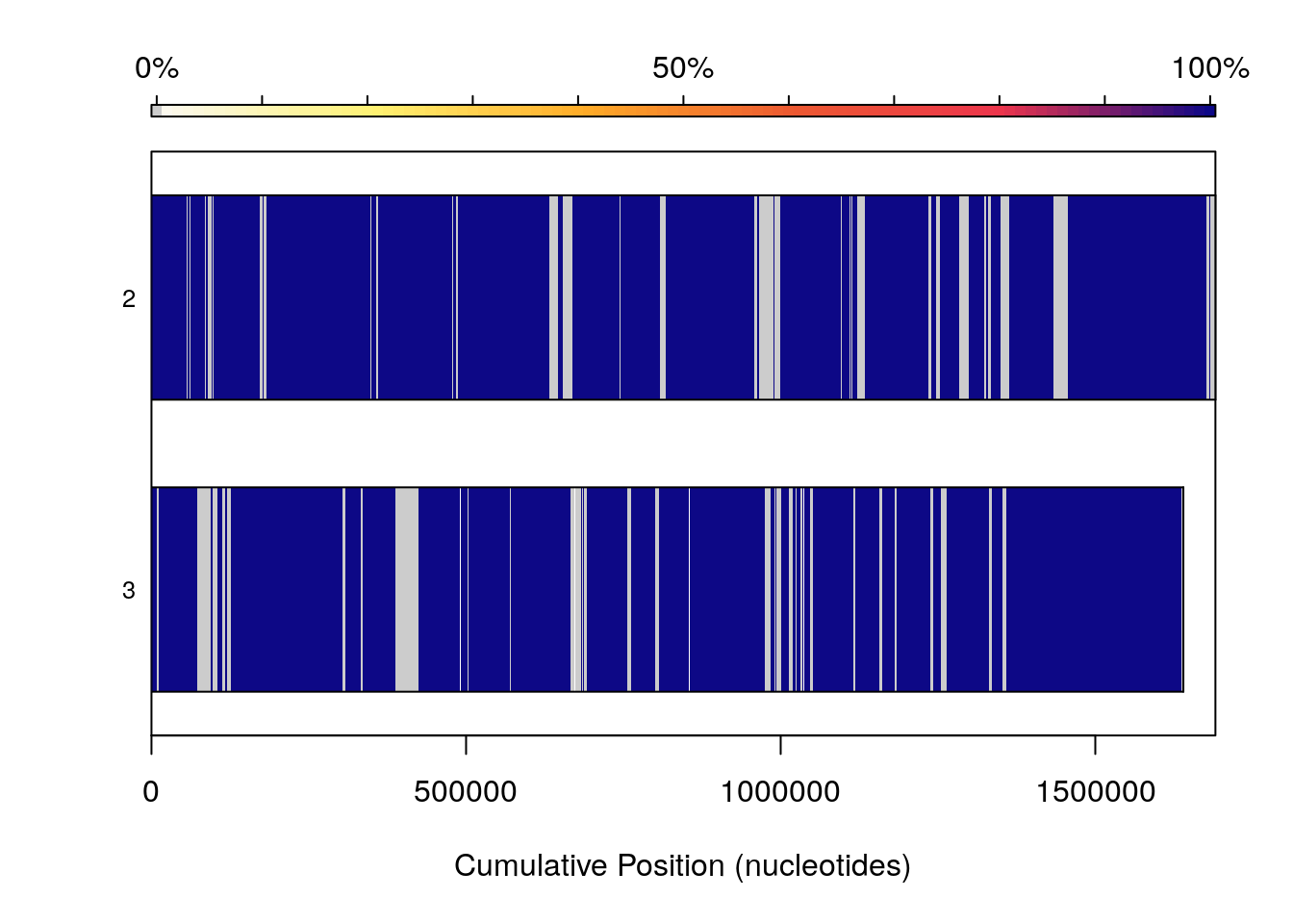

Because visualizing large numbers of syntenic hits in genome sized sequences can be non-trivial, additional commands can be passed to plot in order to modify coloring schemes. neighbor tries to provide each syntenic hit with a unique color, and additionally draws linear connections between them to facilitate better visualization. This can be a useful alternative to the default plotting, if many rearrangements are present in a way that you want to view.

plot(SyntenyObject[2:3, 2:3],
     "neighbor")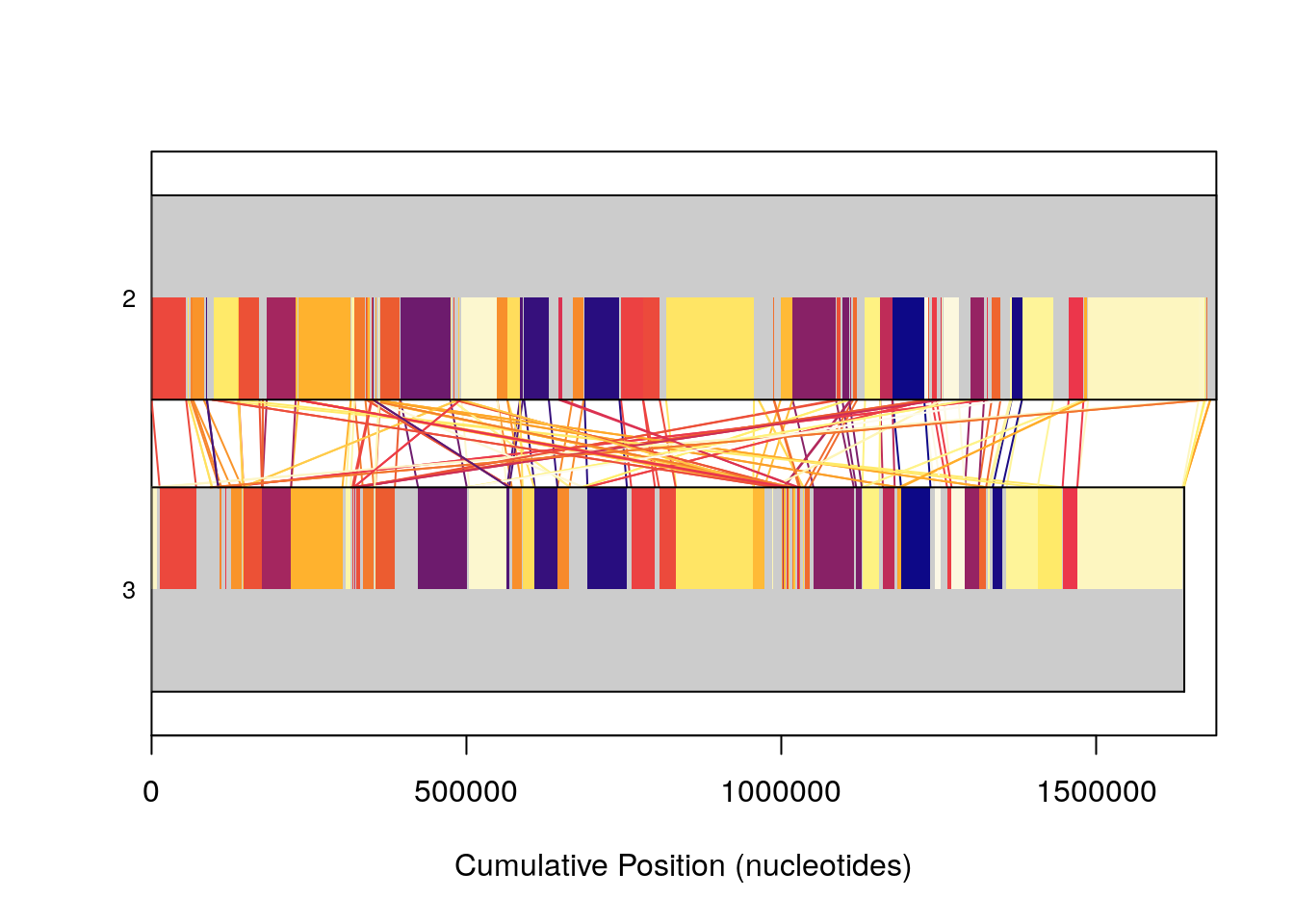

Plotting is a useful tool in analzying sequence data, however sometimes plots of genome sized sequence data can be a bit overwhelming. Plotting our entire database, 8 sequences, though good at representing the complexity present here in this workshop, can be daunting to make sense of quickly if you are unused to looking at figures of this type frequently.

plot(SyntenyObject,
     "neighbor")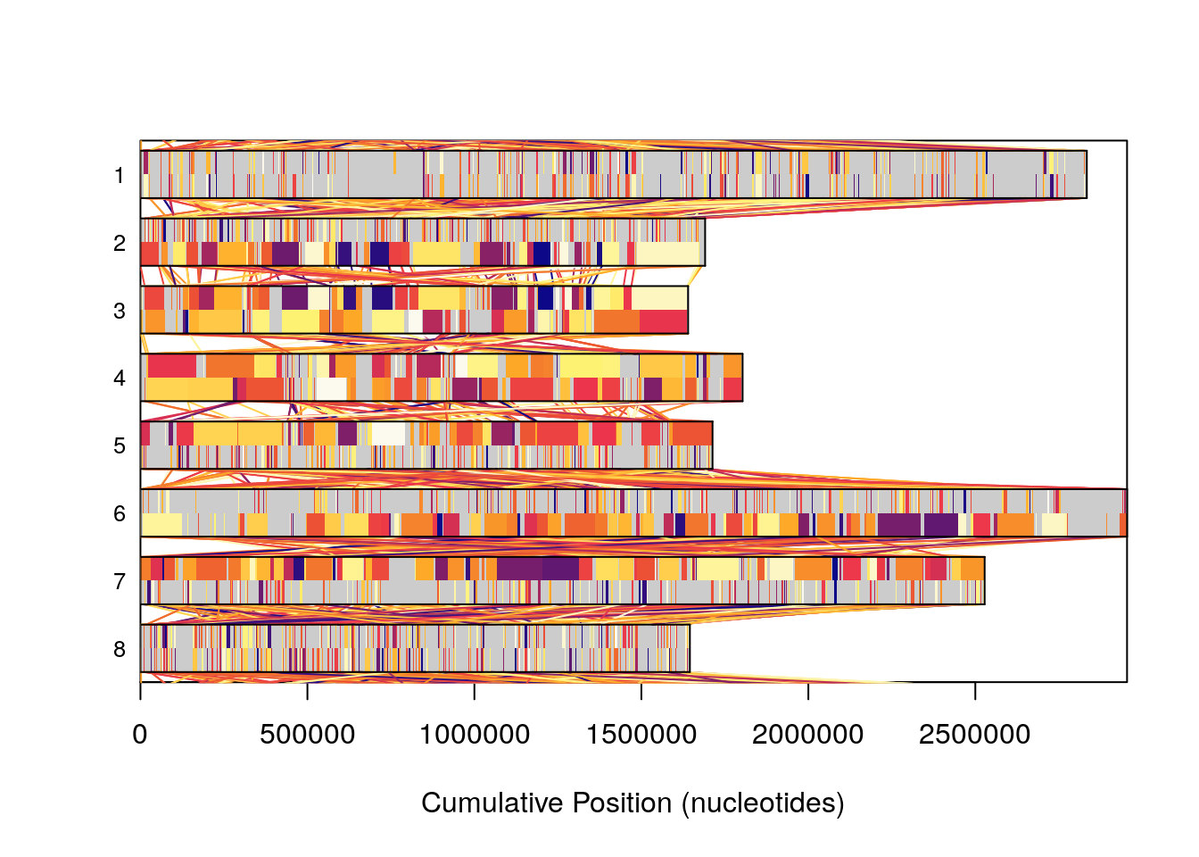

The most useful way to visualize Synteny data in my opinion is through a dot plot, which can be accessed via the pairs(). Dot plots, as explained above, utilize each genome being compared, as an axis in a normal x-y scatter plot. Where a dot - really a very short line, representing a run of nucleotides or amino acids - is shown, that x,y coordinate is a syntenic hit. Hits can also be chained together into blocks of syntenic hits.

pairs(SyntenyObject[2:3, 2:3], labels = GenomeIDs[2:3])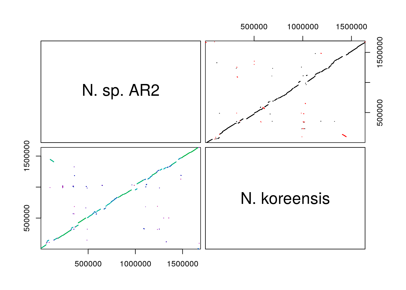

Syntenic hits are shown in the upper left, while syntenic blocks are shown in the bottom left. In the upper triangle,hits in black are co-linear, while hits in red are inverted. In the bottom triangle, blocks are colored by score.

Pairs plots are my personal favorite way to visualize syntenic information, but, they can become overwhelming as the number of genomes compared increases. They provide very clear depictions of rearrangements and inversions.

pairs(SyntenyObject,
      labels = GenomeIDs)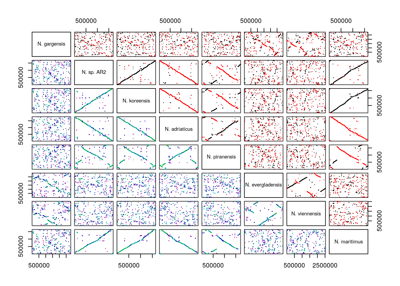

13.2.2.8 Predict homology between genes that are linked by syntenic hits

The FindHomology package contains 5 functions, the second of which is below. NucleotideOverlap takes in an object of class Synteny, and a list of gene calls. We previously generated the object SyntenyObject, using DECIPHER’s function FindSynteny, and a list of gene calls and annotations using GFFParser. Here we will use these two objects to build what is functionally a list of pairs of genes that are linked by syntenic hits. These linking of hits are used as predictions of homology. A single position in the object of class Synteny represents a pairwise comparison between two genomes. The corresponding position in NucleotideOverlap’s output object, is generated from that pairwise comparison, and the gene calls for each genome involved.

This is a fun object to scroll through, but is often very long, representing thousands of paired genes and is not represented well visually, a simple example would be:

Genome 1	Genome 2	# of Nucleotides
Gene A	Gene Z	25L
Gene B	Gene Y	1251L
Gene C	Gene X	145L
Gene …	Gene …	…

The reason we name this “MatrixObject” below is because the shape and dimensions of our data are dependent upon our synteny object. As in, if our Synteny object was built from 5 genomes, that object is a 5 x 5 matrix. NucleotideOverlap accesses the upper triangle of that object to build a 5 x 5 matrix where each position is built from data in the analogous position from the Synteny object. MatrixObject[[1]][1, 2] below was created from SyntenyObject[[1]][1, 2] and so on and so forth.

MatrixObject <- NucleotideOverlap(SyntenyObject = SyntenyObject,
                                  GeneCalls = GeneCalls,
                                  Verbose = TRUE)
#> ===========================================================================
#> Time difference of 1.04628 mins

The function Catalog takes in the output of NucleotideOverlap and returns a list of matrices. These matrices represent agglomerated sets of pairs. The idea being, if gene A in genome 1 was paired by nucleotide overlap to genes B and C in genomes 2 and 3 respectively by NucleotideOverLap, and additionally gene B in genome 2 was similarly paired with gene C in genome 3. With the assumption that these linkages indicate homology, gene A is predicted to be homologous to genes B and C, and gene B is predicted to be homologous to gene C.

Genome 1	Genome 2	Genome 3
Gene A	Gene B	NA
NA	Gene B	Gene C
Gene A	NA	Gene C

Catalog will return every agglomerated set of pairs, of every size possible for the given set of genomes. From a matrix with a single row, indicating a pair of genes that are predicted to have no other homologs anywhere else in the set of genomes, to a large matrix indicating that homologs are located in every genome, and are all predicted to be homologous to each other.

Homologs <- Catalog(MatrixObject,
                    Verbose = TRUE)
#> ===========================================================================
#> Time difference of 1.901221 mins

We can visualize this object as a histogram of the size of these agglomerations, by the number of pairs included in each agglomerated group. Where 1 represents pairs of genes where neither gene is linked to any other gene, from other genomes. Where 28 in this case represents fully linked sets of pairs, where each gene in the set is predicted to be a homolog of every other gene in the set.

hist(sapply(Homologs,
            function(x) nrow(x)),
     main = "Size of Agglomerations",
     ylab = "Number of Sets",
     xlab = "Numer of Gene Pairs",
     breaks = 27L)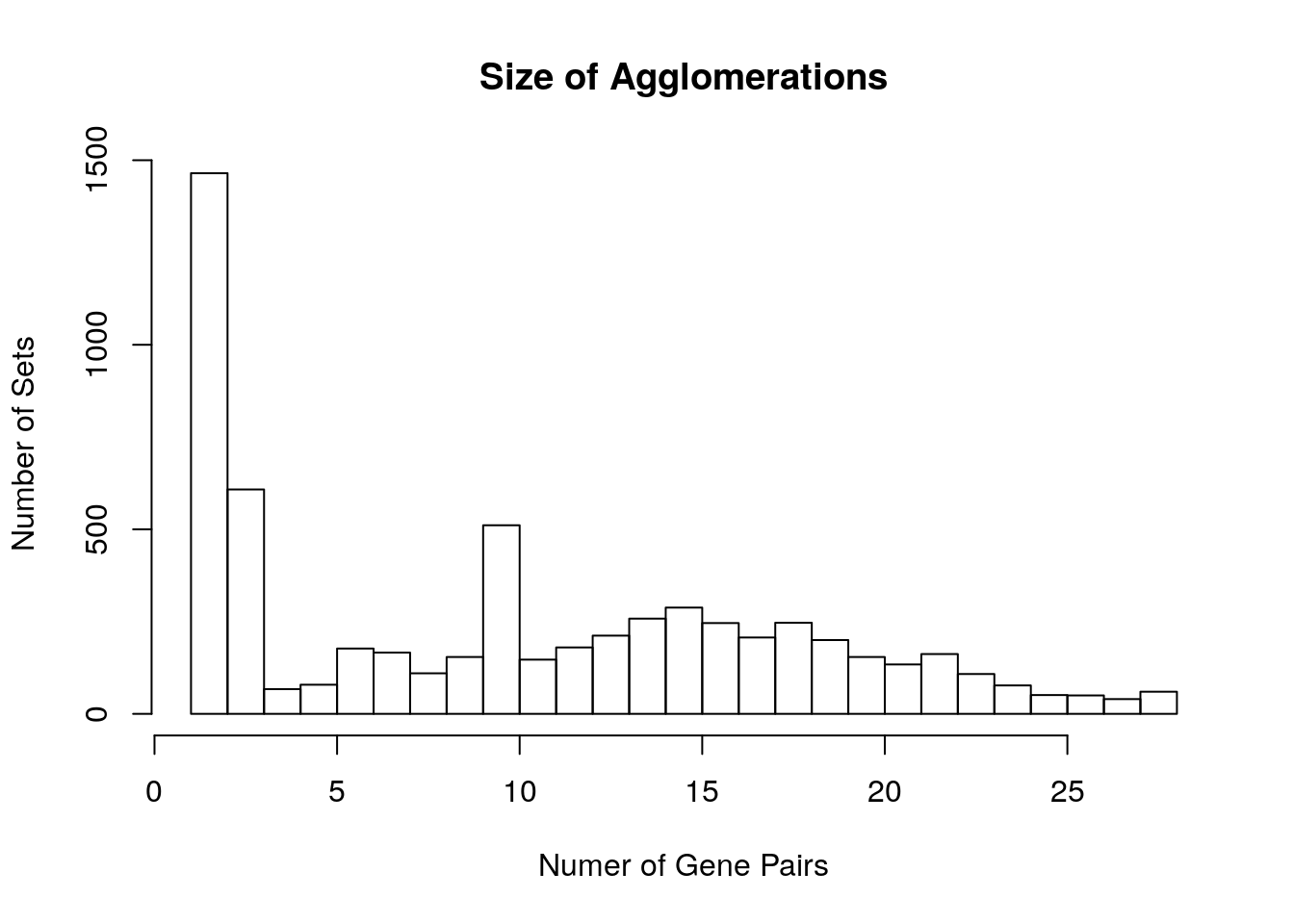

We can collect these fully linked sets. For any N number of genomes, a set of genes where each genome contains a homolog, and those homologs in turn have agreeing homologs in every other genome, the number of rows of this matrix will be N * (N-1) / 2.

You could additionally query this list for any other presence absence pattern that you may be interested in, especially if it can be easily linked to the number of rows in each matrix.

MaxRows <- max(sapply(Homologs,
                      function(x) nrow(x)))
CoreSet <- which(sapply(Homologs,
                        function(x) nrow(x)) == MaxRows)

The second to last function in FindHomology, CoreAligner, collects the genes in these sets, from their respective genomes, aligns the respective sets, and then concatonates the alignments. Creating a concatonated core genome for this set of genomes. This function relies on a few DECIPHER functions internally, and utilizes DECIPHER’s database functionality to perform that collection of genes. Additionally, we can use a few more DECIPHER functions to create a distance matrix from our concatonated core genome, and create a phylogenetic tree from that concatonated core.

CoreGenome <- CoreAligner(Homologs[CoreSet],
                          PATH = DBPath,
                          GeneCalls = GeneCalls,
                          Verbose = TRUE)
#> ===========================================================================
#> Time difference of 33.67113 secs
CoreDist <- DistanceMatrix(myXStringSet = CoreGenome,
                           verbose = FALSE,
                           correction = "Jukes-Cantor")
CoreDend <- IdClusters(myDistMatrix = CoreDist,
                       myXStringSet = CoreGenome,
                       method = "NJ",
                       verbose = FALSE,
                       showPlot = TRUE,
                       type = "dendrogram")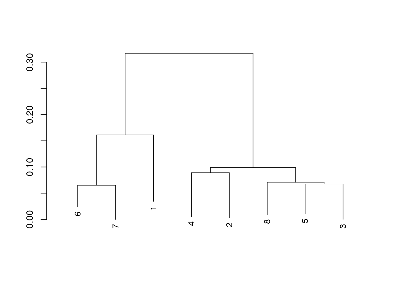

We can now finally tidy up our workspace and unlink our temp file.

unlink(DBPath)

We are also interested in the pan genome, and FindHomolog’s LogicalPan function allows us to utilize the Homologs object, and the list of GeneCall dataframes, to create a presence absence matrix of the pan genome.

PanGenomeMatrix <- LogicalPan(HomologList = Homologs,
                              GeneCalls = GeneCalls,
                              Verbose = TRUE,
                              Plot = FALSE)
#> ===========================================================================
#> Time difference of 1.028313 secs

We can visualize this matrix if we so choose.

image(t(PanGenomeMatrix), col = c("white", "blue"),
      main = "Presence Absence")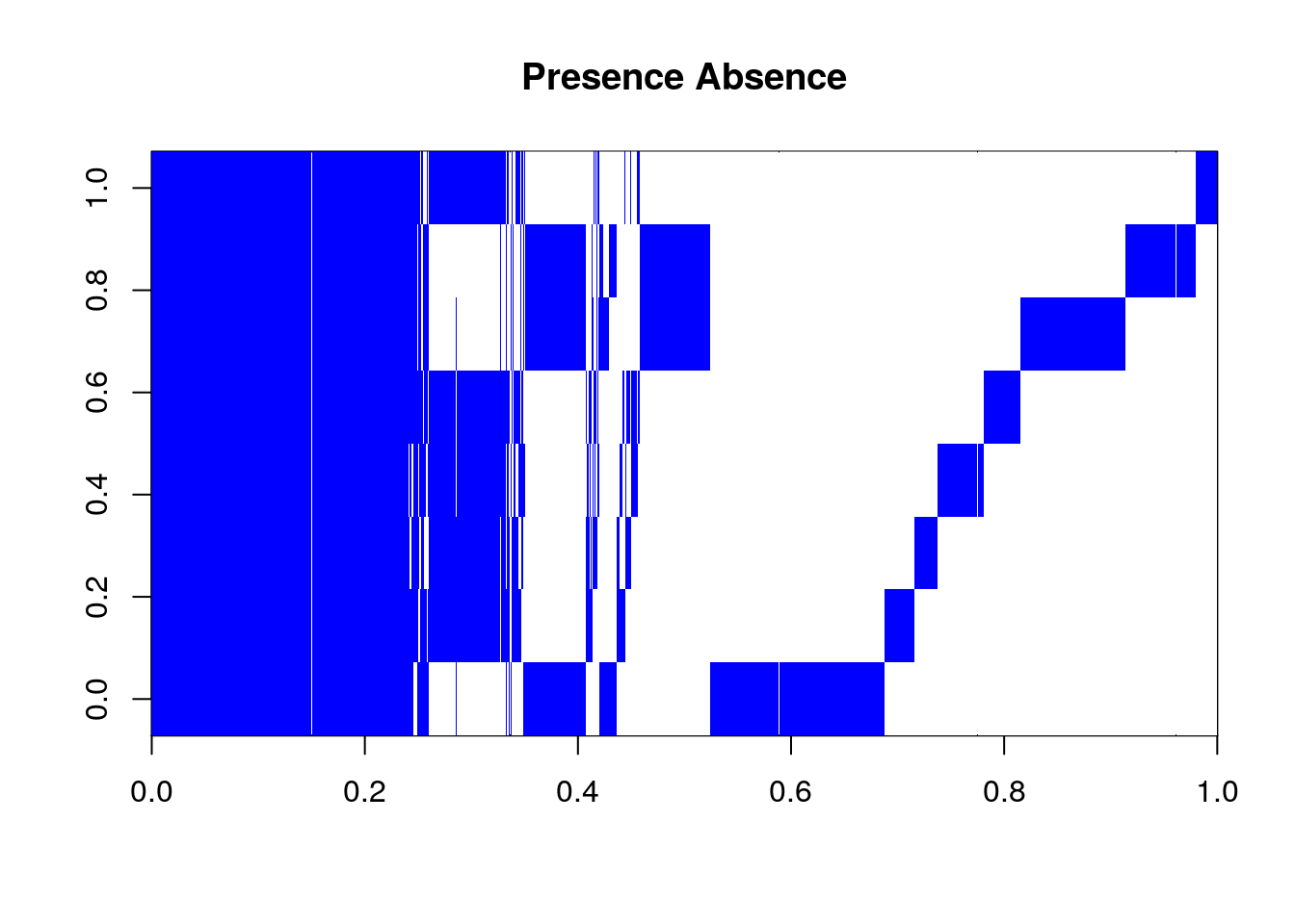

PanGenomeMatrix represents every homolog set, and every singleton gene in our genomes.

This matrix is constructed from the object Homologs which is a list of matrices. Each matrix represents of a set of predicted homologous pairs. Some of the sets are small, say a single pair. Some are large, encompassing genes in every genome in our set. However, the one thing this matrix is missing is singleton genes from each genome. Genes that have no predicted homologs by our method.

And we can create a dendrogram from this matrix.

PanGenome <- dist(PanGenomeMatrix,
                  method = "binary")
PanDend <- IdClusters(myDistMatrix = PanGenome,
                      method = "NJ",
                      type = "dendrogram",
                      showPlot = TRUE,
                      verbose = FALSE)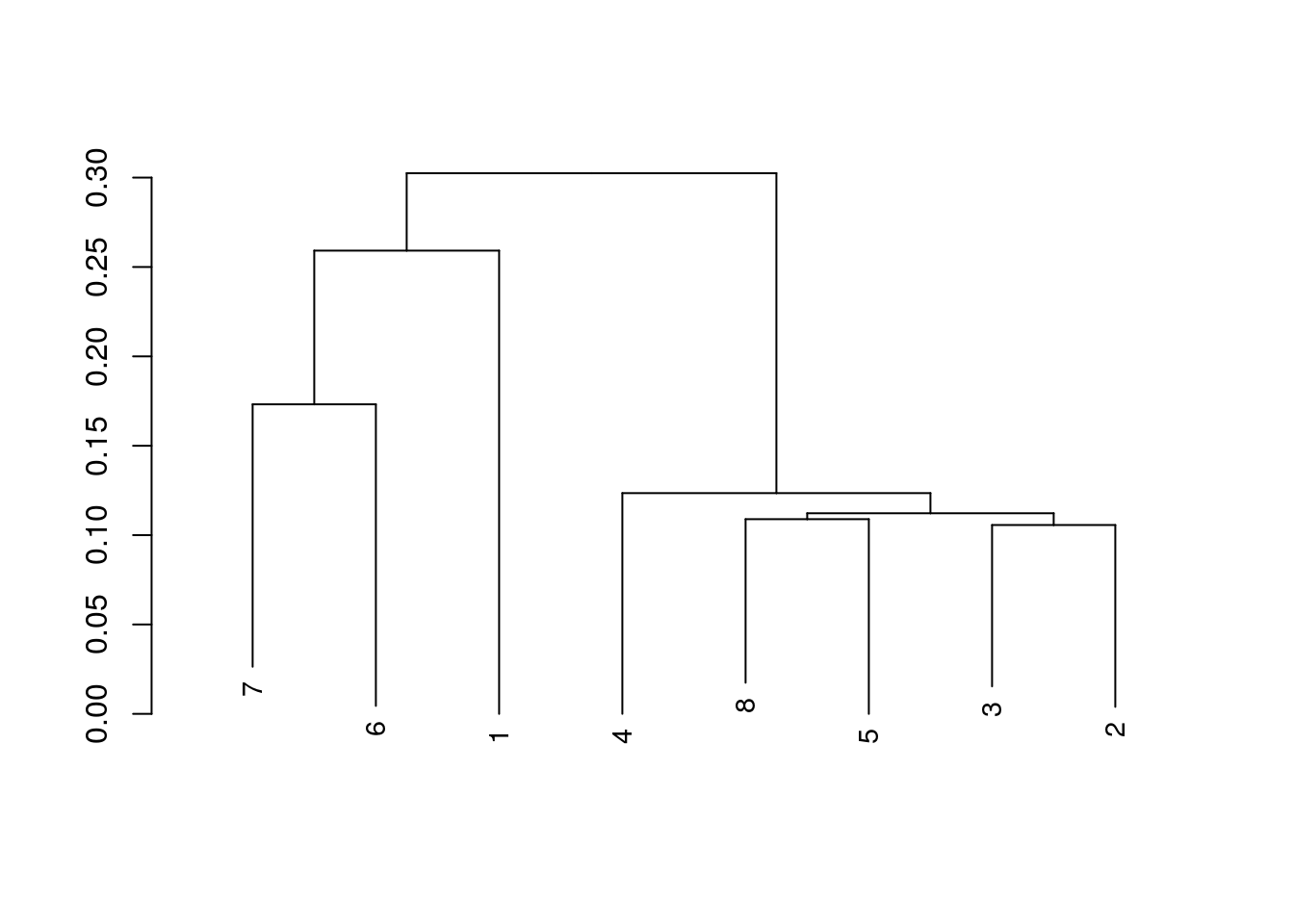

We can, additionally, create a simple tangleogram from these two phylogenetic trees. Allowing a comparison of the core, and pan genomes. The core is on the left, while the pan is on the right.

tf1 <- tempfile()
tf2 <- tempfile()

WriteDendrogram(x =PanDend,
                file = tf1)

WriteDendrogram(x = CoreDend,
                file = tf2)

unlink(tf1)
unlink(tf2)
layout(matrix(1:2, nrow = 1L))
p <- par(mar = c(5, 2, 1, 2))
plot(CoreDend, horiz = TRUE, leaflab = "none")
par(mar = c(5, 2, 1, 2))
plot(PanDend, horiz = TRUE, xlim = c(0, attr(PanDend, "height")), leaflab = "none")
C.Ord <- unlist(CoreDend)
P.Ord <- unlist(PanDend)
segments(-0.10, seq_along(C.Ord), -0.01, match(C.Ord, P.Ord), xpd = NA, col = "blue")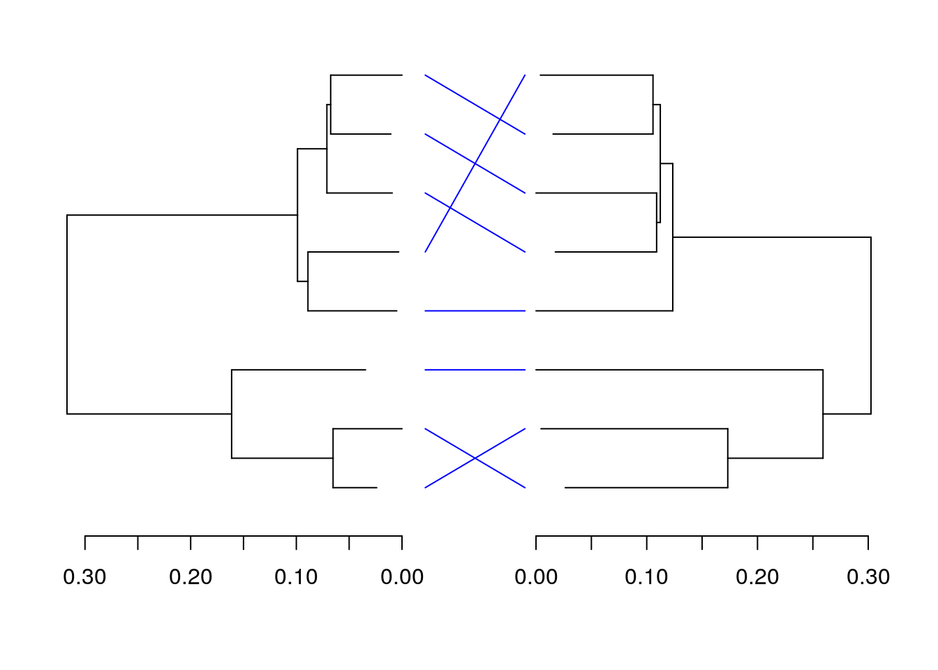

par(p)

The proposition at the beginning of this workshop was that a specific set of genes, that may not normally be included in a core genome, could be included in the core genome, for this set of Archaea. Specifically, genes involved in some of the unusual chemistry that Archaea do with their lipids. If we wanted to really prove this, a significant amount of lab work would also be required. However we can collect the annotations for all of the sets of homologs that have been predicted, and see how much these annotations agree, and if any of these annotations provide evidence for our proposition.

CoreGenes <- matrix(data = NA_integer_,
                        ncol = length(GeneCalls),
                        nrow = length(CoreSet))
CoreAnnotations <- matrix(data = NA_character_,
                              ncol = length(GeneCalls),
                              nrow = length(CoreSet))
for (i in seq_len(ncol(CoreGenes))) {
  for (j in seq_len(nrow(CoreGenes))) {
    CoreGenes[j, i] <- unique(Homologs[CoreSet[j]][[1]][, i])[!is.na(unique(Homologs[CoreSet[j]][[1]][, i]))]
    CoreAnnotations[j, i] <- GeneCalls[[i]][CoreGenes[j, i], "Annotation"]
  }
}

CoreAnnotations <- t(CoreAnnotations)
CoreAnnotations <- data.frame(CoreAnnotations,
                                  stringsAsFactors = FALSE)

The annotations for each core set can now be viewed. Some provide near-universal agreement, while others indicate genes of similar family and function, but potentially not an exact match.

CoreAnnotations[, c(1L, 3L)]
#>                                X1                                       X3
#> 1        acetoacetyl-CoA thiolase    DNA-directed RNA polymerase subunit H
#> 2 propanoyl-CoA C-acyltransferase                      RNA polymerase Rpb5
#> 3 propanoyl-CoA C-acyltransferase                      RNA polymerase Rpb5
#> 4        acetoacetyl-CoA thiolase    DNA-directed RNA polymerase subunit H
#> 5        acetoacetyl-CoA thiolase    DNA-directed RNA polymerase subunit H
#> 6    acetyl-CoA acetyltransferase DNA-directed RNA polymerase%2C subunit H
#> 7        acetoacetyl-CoA thiolase    DNA-directed RNA polymerase subunit H
#> 8 Propanoyl-CoA C-acyltransferase                      RNA polymerase Rpb5

There are 60 of these!

CoreAnnotations[, 2L]
#> [1] "ribonucleoside-diphosphate reductase"                               
#> [2] "ribonucleoside-diphosphate reductase%2C adenosylcobalamin-dependent"
#> [3] "ribonucleoside-diphosphate reductase%2C adenosylcobalamin-dependent"
#> [4] "Ribonucleoside-diphosphate reductase"                               
#> [5] "Ribonucleoside-diphosphate reductase"                               
#> [6] "ribonucleoside-diphosphate reductase class II"                      
#> [7] "ribonucleoside-diphosphate reductase"                               
#> [8] "ribonucleoside-diphosphate reductase%2C adenosylcobalamin-dependent"

Now, a little insider baseball is that the unique chemistry we’re interested in is often the chemistry of radicals, especially in biological systems, where the process is tightly controlled by enzymes. A quick perusal of all the sets of annotations provides two sets that support our original hypothesis.

CoreAnnotations[, c(17L, 31L)]
#>                            X17                                 X31
#> 1   radical SAM domain protein putative radical SAM domain protein
#> 2          radical SAM protein                 radical SAM protein
#> 3          radical SAM protein                 radical SAM protein
#> 4   Radical SAM domain protein                 Radical SAM protein
#> 5         hypothetical protein                 Radical SAM protein
#> 6 putative Fe-S oxidoreductase                 Fe-S oxidoreductase
#> 7   radical SAM domain protein putative radical SAM domain protein
#> 8   Radical SAM domain protein          Radical SAM domain protein

This concludes the workshop, as any analysis after this would require work in a wet lab. Hopefully this was a useful showcase for the power of using DECIPHER to analyze sets of genomic data. The package FindHomology is currently located on github, and is still under construction. Upon completion, it will be available on Bioconductor.

Thank you for your time and attention! We hope you learned something, and if you come back to this at a later date and have any questions, concerns, or comments, feel free to email me, or you can tweet at me.