12 240: Fluent genomic data analysis with plyranges
12.1 Instructor names and contact information
- Stuart Lee (lee.s@wehi.edu.au)
- Michael Lawrence (michafla@gmail.com)
12.2 Workshop Description
In this workshop, we will give an overview of how to perform low-level analyses of genomic data using the grammar of genomic data transformation defined in the plyranges package. We will cover:
- introduction to GRanges
- overview of the core verbs for arithmetic, restriction, and aggregation of GRanges objects
- performing joins between GRanges objects
- designing pipelines to quickly explore data from AnnotationHub
- reading BAM and other file types as GRanges objects
The workshop will be a computer lab, in which the participants will be able to ask questions and interact with the instructors.
12.2.1 Pre-requisites
This workshop is self-contained however familiarity with the following would be useful:
- plyranges vignette
- the GenomicRanges and IRanges packages
- tidyverse approaches to data analysis
12.2.2 Workshop Participation
Students will work through an Rmarkdown document while the instructors respond to any questions they have.
12.2.3 R / Bioconductor packages used
- plyranges
- airway
- AnnotationHub
- GenomicRanges
- IRanges
- S4Vectors
12.2.4 Time outline
| Activity | Time |
|---|---|
| Overview of GRanges | 5m |
| The plyranges grammar | 20m |
| I/O and data pipelines | 20m |
12.3 Workshop goals and objectives
12.3.1 Learning goals
- Understand that GRanges follows tidy data principles
- Apply the plyranges grammar to genomic data analysis
12.3.2 Learning objectives
- Use AnnotationHub to find and summarise data
- Read files into R as GRanges objects
- Perform coverage analysis
- Build data pipelines for analysis based on GRanges
12.4 Workshop
12.5 Introduction
12.5.1 What is plyranges?
The plyranges package is a domain specific language (DSL) built on top of the IRanges and GenomicRanges packages (Lee, Cook, and Lawrence (2018); Lawrence et al. (2013)). It is designed to quickly and coherently analyse genomic data in the form of GRanges objects (more on those later!) and from a wide variety of genomic data file types. For users who are familiar with the tidyverse, the grammar that plyranges implements will look familiar but with a few modifications for genomic specific tasks.
12.5.2 Why use plyranges?
The grammar that plyranges develops is helpful for reasoning about genomics data analysis, and provides a way of developing short readable analysis pipelines. We have tried to emphasise consistency and code readability by following the design principles outlined by Green and Petre (1996).
One of the goals of plyranges is to provide an alternative entry point to analysing genomics data with Bioconductor, especially for R beginners and R users who are more familiar with the tidyverse approach to data analysis. As a result, we have de-emphasised the use of more complicated data structures provided by core Bioconductor packages that are useful for programming with.
12.5.3 Who is this workshop for?
This workshop is intended for new users of Bioconductor, users who are interested to learn about grammar based approaches for data analysis, and users who are interested in learning how to use R to perform analyses like those available in the command line packages BEDTools (Quinlan and Hall (2010)).
If that’s you, let’s begin!
12.6 Setup
To participate in this workshop you’ll need to have R >= 3.5 and install the plyranges, AnnotationHub, and airway Bioconductor 3.7 packages (Morgan (2018); Love (2018)). You can achieve this by installing the BiocManager package from CRAN, loading it then running the install command:
install.packages("BiocManager")
library(BiocManager)
install(c("plyranges", "AnnotationHub", "airway"))
12.7 What are GRanges objects?
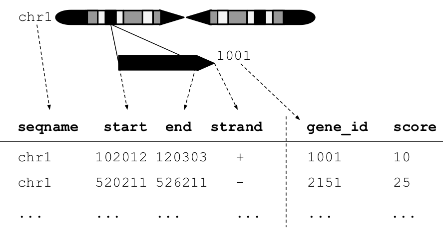
Figure 4.1: An illustration of a GRanges data object for a single sample from an RNA-seq experiment. The core components of the object include a seqname column (representing the chromosome), a ranges column which consists of start and end coordinates for a genomic region, and a strand identifier (either positive, negative, or unstranded). Metadata are included as columns to the right of the dotted line as annotations (gene-id) or range level covariates (score).
The plyranges package is built on the core Bioconductor data structure GRanges. It is very similar to the base R data.frame but with appropriate semantics for a genomics experiment: it has fixed columns for the chromosome, start and end coordinates, and the strand, along with an arbitrary set of additional columns, consisting of measurements or metadata specific to the data type or experiment (figure 4.1).
GRanges balances flexibility with formal constraints, so that it is applicable to virtually any genomic workflow, while also being semantically rich enough to support high-level operations on genomic ranges. As a core data structure, GRanges enables compatibility between plyranges and the rest of Bioconductor.
Since a GRanges object is similar to a data.frame, we can use plyranges to construct a GRanges object from a data.frame. We’ll start by supposing we have a data.frame of genes from the yeast genome:
library(plyranges, quietly = TRUE)
genes <- data.frame(seqnames = "VI",
                    start = c(3322, 3030, 1437,  5066, 6426, 836),
                    end = c(3846, 3338, 2615, 5521, 7565, 1363),
                    strand = c("-", "-", "-", "+", "+", "+"),
                    gene_id=c("YFL064C", "YFL065C", "YFL066C",
                              "YFL063W", "YFL062W", "YFL067W"),
                    stringsAsFactors = FALSE)
gr <- as_granges(genes)
gr
#> GRanges object with 6 ranges and 1 metadata column:
#>       seqnames    ranges strand |     gene_id
#>          <Rle> <IRanges>  <Rle> | <character>
#>   [1]       VI 3322-3846      - |     YFL064C
#>   [2]       VI 3030-3338      - |     YFL065C
#>   [3]       VI 1437-2615      - |     YFL066C
#>   [4]       VI 5066-5521      + |     YFL063W
#>   [5]       VI 6426-7565      + |     YFL062W
#>   [6]       VI  836-1363      + |     YFL067W
#>   -------
#>   seqinfo: 1 sequence from an unspecified genome; no seqlengths
The as_granges method takes a data.frame and allows you to quickly convert it to a GRanges object (and can you can also specify which columns in the data.frame correspond to the columns in the GRanges).
A GRanges object follows tidy data principles: it is a rectangular table corresponding to a single biological context (Wickham (2014)). Each row contains a single observation and each column is a variable describing the observations. In the example above, each row corresponds to a single gene, and each column contains information about those genes. As GRanges are tidy, we have constructed plyranges to follow and extend the grammar in the R package dplyr.
12.8 The Grammar
Here we provide a quick overview of the functions available in plyranges and illustrate their use with some toy examples (see 12.11 for an overview). In the final section we provide two worked examples (with exercises) that show you can use plyranges to explore publicly available genomics data and perform coverage analysis of BAM files.
12.8.1 Core verbs
The plyranges grammar is simply a set of verbs that define actions to be performed on a GRanges (for a complete list see the appendix). Verbs can be composed together using the pipe operator, %>%, which can be read as ‘then’. Here’s a simple pipeline: first we will add two columns, one corresponding to the gene_type and another with the GC content (which we make up by drawing from a uniform distribution). Second we will remove genes if they have a width less than 400bp.
set.seed(2018-07-28)
gr2 <- gr %>%
  mutate(gene_type = "ORF",
         gc_content = runif(n())) %>%
  filter(width > 400)
gr2
#> GRanges object with 5 ranges and 3 metadata columns:
#>       seqnames    ranges strand |     gene_id   gene_type
#>          <Rle> <IRanges>  <Rle> | <character> <character>
#>   [1]       VI 3322-3846      - |     YFL064C         ORF
#>   [2]       VI 1437-2615      - |     YFL066C         ORF
#>   [3]       VI 5066-5521      + |     YFL063W         ORF
#>   [4]       VI 6426-7565      + |     YFL062W         ORF
#>   [5]       VI  836-1363      + |     YFL067W         ORF
#>              gc_content
#>               <numeric>
#>   [1]  0.49319754820317
#>   [2] 0.216616344172508
#>   [3] 0.747259315103292
#>   [4] 0.907683959929273
#>   [5] 0.221016310621053
#>   -------
#>   seqinfo: 1 sequence from an unspecified genome; no seqlengths
The mutate() function is used to add columns, here we’ve added one column called gene_type where all values are set to “ORF” (standing for open reading frame) and another called gc_content with random uniform values. The n() operator returns the number of ranges in GRanges object, but can only be evaluated inside of one of the plyranges verbs.
The filter() operation returns ranges if the expression evaluates to TRUE. Multiple expressions can be composed together and will be evaluated as &
gr2 %>%
  filter(strand == "+", gc_content > 0.5)
#> GRanges object with 2 ranges and 3 metadata columns:
#>       seqnames    ranges strand |     gene_id   gene_type
#>          <Rle> <IRanges>  <Rle> | <character> <character>
#>   [1]       VI 5066-5521      + |     YFL063W         ORF
#>   [2]       VI 6426-7565      + |     YFL062W         ORF
#>              gc_content
#>               <numeric>
#>   [1] 0.747259315103292
#>   [2] 0.907683959929273
#>   -------
#>   seqinfo: 1 sequence from an unspecified genome; no seqlengths
# is the same as using `&`
gr2 %>%
  filter(strand == "+" & gc_content > 0.5)
#> GRanges object with 2 ranges and 3 metadata columns:
#>       seqnames    ranges strand |     gene_id   gene_type
#>          <Rle> <IRanges>  <Rle> | <character> <character>
#>   [1]       VI 5066-5521      + |     YFL063W         ORF
#>   [2]       VI 6426-7565      + |     YFL062W         ORF
#>              gc_content
#>               <numeric>
#>   [1] 0.747259315103292
#>   [2] 0.907683959929273
#>   -------
#>   seqinfo: 1 sequence from an unspecified genome; no seqlengths
# but different from using or '|'
gr2 %>%
  filter(strand == "+" | gc_content > 0.5)
#> GRanges object with 3 ranges and 3 metadata columns:
#>       seqnames    ranges strand |     gene_id   gene_type
#>          <Rle> <IRanges>  <Rle> | <character> <character>
#>   [1]       VI 5066-5521      + |     YFL063W         ORF
#>   [2]       VI 6426-7565      + |     YFL062W         ORF
#>   [3]       VI  836-1363      + |     YFL067W         ORF
#>              gc_content
#>               <numeric>
#>   [1] 0.747259315103292
#>   [2] 0.907683959929273
#>   [3] 0.221016310621053
#>   -------
#>   seqinfo: 1 sequence from an unspecified genome; no seqlengths
Now that we have some measurements over our genes, we are most likely interested in performing the favourite tasks of a biological data scientist: taking averages and counting. This is achieved with the summarise() verb which will return a DataFrame object (Why is this the case?).
gr2 %>%
  summarise(avg_gc = mean(gc_content),
            n = n())
#> DataFrame with 1 row and 2 columns
#>              avg_gc         n
#>           <numeric> <integer>
#> 1 0.517154695605859         5
which isn’t very exciting when performed without summarise()’s best friend the group_by() operator:
gr2 %>%
  group_by(strand) %>%
  summarise(avg_gc = mean(gc_content),
            n = n())
#> DataFrame with 2 rows and 3 columns
#>   strand            avg_gc         n
#>    <Rle>         <numeric> <integer>
#> 1      + 0.625319861884539         3
#> 2      - 0.354906946187839         2
The group_by() operator causes plyranges verbs to behave differently. Instead of acting on all the ranges in a GRanges object, the verbs act within each group of ranges defined by the values in the grouping column(s). The group_by() operator does not change the appearance the of a GRanges object (well for the most part):
by_strand <- gr2 %>%
  group_by(strand)
by_strand
#> GRanges object with 5 ranges and 3 metadata columns:
#> Groups: strand [2]
#>       seqnames    ranges strand |     gene_id   gene_type
#>          <Rle> <IRanges>  <Rle> | <character> <character>
#>   [1]       VI 3322-3846      - |     YFL064C         ORF
#>   [2]       VI 1437-2615      - |     YFL066C         ORF
#>   [3]       VI 5066-5521      + |     YFL063W         ORF
#>   [4]       VI 6426-7565      + |     YFL062W         ORF
#>   [5]       VI  836-1363      + |     YFL067W         ORF
#>              gc_content
#>               <numeric>
#>   [1]  0.49319754820317
#>   [2] 0.216616344172508
#>   [3] 0.747259315103292
#>   [4] 0.907683959929273
#>   [5] 0.221016310621053
#>   -------
#>   seqinfo: 1 sequence from an unspecified genome; no seqlengths
Now any verb we apply to our grouped GRanges, acts on each partition:
by_strand %>%
  filter(n() > 2)
#> GRanges object with 3 ranges and 3 metadata columns:
#> Groups: strand [1]
#>       seqnames    ranges strand |     gene_id   gene_type
#>          <Rle> <IRanges>  <Rle> | <character> <character>
#>   [1]       VI 5066-5521      + |     YFL063W         ORF
#>   [2]       VI 6426-7565      + |     YFL062W         ORF
#>   [3]       VI  836-1363      + |     YFL067W         ORF
#>              gc_content
#>               <numeric>
#>   [1] 0.747259315103292
#>   [2] 0.907683959929273
#>   [3] 0.221016310621053
#>   -------
#>   seqinfo: 1 sequence from an unspecified genome; no seqlengths
by_strand %>%
  mutate(avg_gc_strand = mean(gc_content))
#> GRanges object with 5 ranges and 4 metadata columns:
#> Groups: strand [2]
#>       seqnames    ranges strand |     gene_id   gene_type
#>          <Rle> <IRanges>  <Rle> | <character> <character>
#>   [1]       VI 3322-3846      - |     YFL064C         ORF
#>   [2]       VI 1437-2615      - |     YFL066C         ORF
#>   [3]       VI 5066-5521      + |     YFL063W         ORF
#>   [4]       VI 6426-7565      + |     YFL062W         ORF
#>   [5]       VI  836-1363      + |     YFL067W         ORF
#>              gc_content     avg_gc_strand
#>               <numeric>         <numeric>
#>   [1]  0.49319754820317 0.354906946187839
#>   [2] 0.216616344172508 0.354906946187839
#>   [3] 0.747259315103292 0.625319861884539
#>   [4] 0.907683959929273 0.625319861884539
#>   [5] 0.221016310621053 0.625319861884539
#>   -------
#>   seqinfo: 1 sequence from an unspecified genome; no seqlengths
To remove grouping use the ungroup() verb:
by_strand %>%
  ungroup()
#> GRanges object with 5 ranges and 3 metadata columns:
#>       seqnames    ranges strand |     gene_id   gene_type
#>          <Rle> <IRanges>  <Rle> | <character> <character>
#>   [1]       VI 3322-3846      - |     YFL064C         ORF
#>   [2]       VI 1437-2615      - |     YFL066C         ORF
#>   [3]       VI 5066-5521      + |     YFL063W         ORF
#>   [4]       VI 6426-7565      + |     YFL062W         ORF
#>   [5]       VI  836-1363      + |     YFL067W         ORF
#>              gc_content
#>               <numeric>
#>   [1]  0.49319754820317
#>   [2] 0.216616344172508
#>   [3] 0.747259315103292
#>   [4] 0.907683959929273
#>   [5] 0.221016310621053
#>   -------
#>   seqinfo: 1 sequence from an unspecified genome; no seqlengths
Finally, metadata columns can be selected using the select() verb:
gr2 %>%
  select(gene_id, gene_type)
#> GRanges object with 5 ranges and 2 metadata columns:
#>       seqnames    ranges strand |     gene_id   gene_type
#>          <Rle> <IRanges>  <Rle> | <character> <character>
#>   [1]       VI 3322-3846      - |     YFL064C         ORF
#>   [2]       VI 1437-2615      - |     YFL066C         ORF
#>   [3]       VI 5066-5521      + |     YFL063W         ORF
#>   [4]       VI 6426-7565      + |     YFL062W         ORF
#>   [5]       VI  836-1363      + |     YFL067W         ORF
#>   -------
#>   seqinfo: 1 sequence from an unspecified genome; no seqlengths
# is the same as not selecting gc_content
gr2 %>%
  select(-gc_content)
#> GRanges object with 5 ranges and 2 metadata columns:
#>       seqnames    ranges strand |     gene_id   gene_type
#>          <Rle> <IRanges>  <Rle> | <character> <character>
#>   [1]       VI 3322-3846      - |     YFL064C         ORF
#>   [2]       VI 1437-2615      - |     YFL066C         ORF
#>   [3]       VI 5066-5521      + |     YFL063W         ORF
#>   [4]       VI 6426-7565      + |     YFL062W         ORF
#>   [5]       VI  836-1363      + |     YFL067W         ORF
#>   -------
#>   seqinfo: 1 sequence from an unspecified genome; no seqlengths
# you can also select by metadata column index
gr2 %>%
  select(1:2)
#> GRanges object with 5 ranges and 2 metadata columns:
#>       seqnames    ranges strand |     gene_id   gene_type
#>          <Rle> <IRanges>  <Rle> | <character> <character>
#>   [1]       VI 3322-3846      - |     YFL064C         ORF
#>   [2]       VI 1437-2615      - |     YFL066C         ORF
#>   [3]       VI 5066-5521      + |     YFL063W         ORF
#>   [4]       VI 6426-7565      + |     YFL062W         ORF
#>   [5]       VI  836-1363      + |     YFL067W         ORF
#>   -------
#>   seqinfo: 1 sequence from an unspecified genome; no seqlengths
12.8.2 Verbs specific to GRanges
We have seen how you can perform restriction and aggregation on GRanges, but what about specific actions for genomics data analysis, like arithmetic, nearest neighbours or finding overlaps?
12.8.2.1 Arithmetic
Arithmetic operations transform range coordinates, as defined by their start, end and width columns. These three variables are mutually dependent so we have to take care when modifying them. For example, changing the width column needs to change either the start, end or both to preserve integrity of the GRanges:
# by default setting width will fix the starting coordinate
gr %>%
  mutate(width = width + 1)
#> GRanges object with 6 ranges and 1 metadata column:
#>       seqnames    ranges strand |     gene_id
#>          <Rle> <IRanges>  <Rle> | <character>
#>   [1]       VI 3322-3847      - |     YFL064C
#>   [2]       VI 3030-3339      - |     YFL065C
#>   [3]       VI 1437-2616      - |     YFL066C
#>   [4]       VI 5066-5522      + |     YFL063W
#>   [5]       VI 6426-7566      + |     YFL062W
#>   [6]       VI  836-1364      + |     YFL067W
#>   -------
#>   seqinfo: 1 sequence from an unspecified genome; no seqlengths
We introduce the anchor_direction() operator to clarify these modifications. Supported anchor points include the start anchor_start(), end anchor_end() and midpoint anchor_center():
gr %>%
  anchor_end() %>%
  mutate(width = width * 2)
#> GRanges object with 6 ranges and 1 metadata column:
#>       seqnames    ranges strand |     gene_id
#>          <Rle> <IRanges>  <Rle> | <character>
#>   [1]       VI 2797-3846      - |     YFL064C
#>   [2]       VI 2721-3338      - |     YFL065C
#>   [3]       VI  258-2615      - |     YFL066C
#>   [4]       VI 4610-5521      + |     YFL063W
#>   [5]       VI 5286-7565      + |     YFL062W
#>   [6]       VI  308-1363      + |     YFL067W
#>   -------
#>   seqinfo: 1 sequence from an unspecified genome; no seqlengths

gr %>%
  anchor_center() %>%
  mutate(width = width * 2)
#> GRanges object with 6 ranges and 1 metadata column:
#>       seqnames    ranges strand |     gene_id
#>          <Rle> <IRanges>  <Rle> | <character>
#>   [1]       VI 3059-4108      - |     YFL064C
#>   [2]       VI 2875-3492      - |     YFL065C
#>   [3]       VI  847-3204      - |     YFL066C
#>   [4]       VI 4838-5749      + |     YFL063W
#>   [5]       VI 5856-8135      + |     YFL062W
#>   [6]       VI  572-1627      + |     YFL067W
#>   -------
#>   seqinfo: 1 sequence from an unspecified genome; no seqlengths
Note that the anchoring modifier introduces an important departure from the IRanges and GenomicRanges packages: by default we ignore the strandedness of a GRanges object, and instead we provide verbs that make stranded actions explicit. In this case of anchoring we provide the anchor_3p() and anchor_5p() to perform anchoring on the 3’ and 5’ ends of a range.
The table in the appendix provides a complete list of arithmetic options available in plyranges.
12.8.2.2 Genomic aggregation
There are two verbs that can be used to aggregate over nearest neighbours: reduce_ranges() and disjoin_ranges(). The reduce verb merges overlapping and neighbouring ranges:
gr %>% reduce_ranges()
#> GRanges object with 5 ranges and 0 metadata columns:
#>       seqnames    ranges strand
#>          <Rle> <IRanges>  <Rle>
#>   [1]       VI  836-1363      *
#>   [2]       VI 1437-2615      *
#>   [3]       VI 3030-3846      *
#>   [4]       VI 5066-5521      *
#>   [5]       VI 6426-7565      *
#>   -------
#>   seqinfo: 1 sequence from an unspecified genome; no seqlengths
We could find out which genes are overlapping each other by aggregating over the gene_id column and storing the result in a List column:
gr %>%
  reduce_ranges(gene_id = List(gene_id))
#> GRanges object with 5 ranges and 1 metadata column:
#>       seqnames    ranges strand |         gene_id
#>          <Rle> <IRanges>  <Rle> | <CharacterList>
#>   [1]       VI  836-1363      * |         YFL067W
#>   [2]       VI 1437-2615      * |         YFL066C
#>   [3]       VI 3030-3846      * | YFL065C,YFL064C
#>   [4]       VI 5066-5521      * |         YFL063W
#>   [5]       VI 6426-7565      * |         YFL062W
#>   -------
#>   seqinfo: 1 sequence from an unspecified genome; no seqlengths
The disjoin verb takes the union of end points over all ranges, and results in an expanded range
gr %>%
  disjoin_ranges(gene_id = List(gene_id))
#> GRanges object with 7 ranges and 1 metadata column:
#>       seqnames    ranges strand |         gene_id
#>          <Rle> <IRanges>  <Rle> | <CharacterList>
#>   [1]       VI  836-1363      * |         YFL067W
#>   [2]       VI 1437-2615      * |         YFL066C
#>   [3]       VI 3030-3321      * |         YFL065C
#>   [4]       VI 3322-3338      * | YFL064C,YFL065C
#>   [5]       VI 3339-3846      * |         YFL064C
#>   [6]       VI 5066-5521      * |         YFL063W
#>   [7]       VI 6426-7565      * |         YFL062W
#>   -------
#>   seqinfo: 1 sequence from an unspecified genome; no seqlengths
You may have noticed that the resulting range are now unstranded, to take into account stranded features use the directed prefix.
12.8.2.3 Overlaps
Another important class of operations for genomics data analysis is finding overlaps or nearest neighbours. Here’s where we will introduce the plyranges join operators and the overlap aggregation operators.
Now let’s now suppose we have some additional measurements that we have obtained from a new experiment on yeast. These measurements are for three different replicates and represent single nucleotide or insertion deletion intensities from an array. Our collaborator has given us three different data.frames with the data but they all have names inconsistent with the GRanges data structure. Our goal is to unify these into a single GRanges object with column for each measurement and column for the sample identifier.
Here’s our data:
set.seed(66+105+111+99+49+56)

pos <- sample(1:10000, size = 100)
size <- sample(1:3, size = 100, replace = TRUE)
rep1 <- data.frame(chr = "VI",
                  pos = pos,
                  size = size,
                  X = rnorm(100, mean = 2),
                  Y = rnorm(100, mean = 1))

rep2 <- data.frame(chrom = "VI",
                  st = pos,
                  width = size,
                  X = rnorm(100, mean = 0.5, sd = 3),
                  Y = rnorm(100, sd = 2))

rep3 <- data.frame(chromosome = "VI",
                  start = pos,
                  width = size,
                  X = rnorm(100, mean = 2, sd = 3),
                  Y = rnorm(100, mean = 4, sd = 0.5))
For each replicate we want to construct a GRanges object:
# we can tell as_granges which columns in the data.frame
# are the seqnames, and range coordinates
rep1 <- as_granges(rep1, seqnames = chr, start = pos, width = size)
rep2 <- as_granges(rep2, seqnames = chrom, start = st)
rep3 <- as_granges(rep3, seqnames = chromosome)
And to construct our final GRanges object we can bind all our replicates together:
intensities <- bind_ranges(rep1, rep2, rep3, .id = "replicate")
# sort by the starting coordinate
arrange(intensities, start)
#> GRanges object with 300 ranges and 3 metadata columns:
#>         seqnames    ranges strand |                  X                  Y
#>            <Rle> <IRanges>  <Rle> |          <numeric>          <numeric>
#>     [1]       VI    99-100      * |   2.18077108319727   1.15893283880961
#>     [2]       VI    99-100      * |  -1.14331853023759  -1.84545382593297
#>     [3]       VI    99-100      * |   4.42535734042167   3.53884540635964
#>     [4]       VI   110-111      * |   1.41581829875993 -0.262026041514519
#>     [5]       VI   110-111      * | 0.0203313104969627  -1.18095384044377
#>     ...      ...       ...    ... .                ...                ...
#>   [296]       VI 9671-9673      * |  0.756423808063998  -0.24544579405238
#>   [297]       VI 9671-9673      * |  0.715559817063897    4.6963376859667
#>   [298]       VI 9838-9839      * |   1.83836043312615  0.267996156074214
#>   [299]       VI 9838-9839      * |  -4.62774336616852  -3.45271032367217
#>   [300]       VI 9838-9839      * | -0.285141455604857   4.16118336728783
#>           replicate
#>         <character>
#>     [1]           1
#>     [2]           2
#>     [3]           3
#>     [4]           1
#>     [5]           2
#>     ...         ...
#>   [296]           2
#>   [297]           3
#>   [298]           1
#>   [299]           2
#>   [300]           3
#>   -------
#>   seqinfo: 1 sequence from an unspecified genome; no seqlengths
Now we would like to filter our positions if they overlap one of the genes we have, one way we could achieve this is with the filter_by_overlaps() operator:
olap <- filter_by_overlaps(intensities, gr)
olap
#> GRanges object with 108 ranges and 3 metadata columns:
#>         seqnames    ranges strand |                  X                  Y
#>            <Rle> <IRanges>  <Rle> |          <numeric>          <numeric>
#>     [1]       VI 3300-3302      * |   2.26035109119553   1.06568454447289
#>     [2]       VI 1045-1047      * |   2.21864775104592   1.08876098679654
#>     [3]       VI 3791-3793      * |   2.64672161626967   1.49683387927811
#>     [4]       VI      6503      * |   2.97614069143102 -0.842974371427135
#>     [5]       VI 2613-2615      * |  0.829706619102562   1.00867596057383
#>     ...      ...       ...    ... .                ...                ...
#>   [104]       VI      2288      * |   4.51377823089056   3.98977444171162
#>   [105]       VI      7191      * |  -3.91180888573709    5.0451068476909
#>   [106]       VI      5490      * |    6.8026659440345   4.71157047258809
#>   [107]       VI 5268-5270      * |  -1.40753324511308   4.48936193681021
#>   [108]       VI      7333      * | -0.807795033496545   4.12171733927051
#>           replicate
#>         <character>
#>     [1]           1
#>     [2]           1
#>     [3]           1
#>     [4]           1
#>     [5]           1
#>     ...         ...
#>   [104]           3
#>   [105]           3
#>   [106]           3
#>   [107]           3
#>   [108]           3
#>   -------
#>   seqinfo: 1 sequence from an unspecified genome; no seqlengths
Another option would be to perform a join operation. A join acts on two GRanges objects, a query and a subject. The join operator retains the metadata from the query and subject ranges. All join operators generate a set of hits based on overlap or proximity of ranges and use those hits to merge the two datasets in different ways (figure , provides an overview of the overlap joins). We can further restrict the matching by whether the query is completely within the subject, and adding the directed suffix ensures that matching ranges have the same direction (strand).
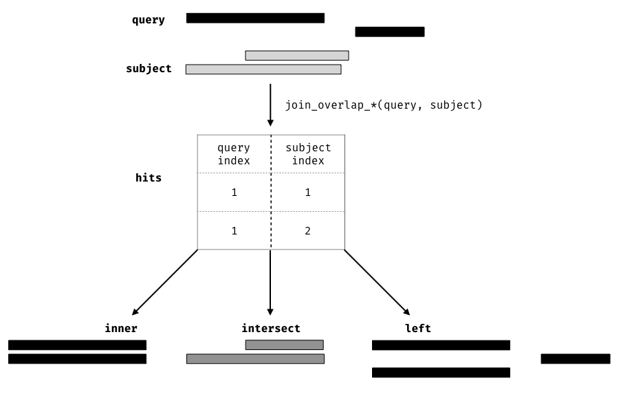
Figure 12.1: Illustration of the three overlap join operators. Each join takes query and subject range as input (black and light gray rectangles, respectively). An index for the join is computed, returning a Hits object, which contains the indices of where the subject overlaps the query range. This index is used to expand the query ranges by where it was ‘hit’ by the subject ranges. The join semantics alter what is returned: for an join the query range is returned for each match, for an the intersection is taken between overlapping ranges, and for a join all query ranges are returned even if the subject range does not overlap them. This principle is gnerally applied through the plyranges package for both overlaps and nearest neighbour operations.
Going back to our example, the overlap inner join will return all intensities that overlap a gene and propagate which gene_id a given intensity belongs to:
olap <- join_overlap_inner(intensities, gr)If we wanted to return all intensities regardless of overlap we could use the left join, and a missing value will be propagated to the gene_id column if there isn’t any overlap.
join_overlap_left(intensities, gr)
#> GRanges object with 300 ranges and 4 metadata columns:
#>         seqnames    ranges strand |                  X                  Y
#>            <Rle> <IRanges>  <Rle> |          <numeric>          <numeric>
#>     [1]       VI 3300-3302      * |   2.26035109119553   1.06568454447289
#>     [2]       VI 1045-1047      * |   2.21864775104592   1.08876098679654
#>     [3]       VI 4206-4207      * |   3.08931723239393    2.4388720191285
#>     [4]       VI 3791-3793      * |   2.64672161626967   1.49683387927811
#>     [5]       VI      6503      * |   2.97614069143102 -0.842974371427135
#>     ...      ...       ...    ... .                ...                ...
#>   [296]       VI 8881-8882      * |   4.15079125018189   4.47576275354234
#>   [297]       VI      7333      * | -0.807795033496545   4.12171733927051
#>   [298]       VI   715-716      * | -0.988759384492962   3.53496809806709
#>   [299]       VI   426-428      * |   10.5245928564545   3.52355010049711
#>   [300]       VI 9187-9188      * |   1.15204426681652   4.12867380190036
#>           replicate     gene_id
#>         <character> <character>
#>     [1]           1     YFL065C
#>     [2]           1     YFL067W
#>     [3]           1        <NA>
#>     [4]           1     YFL064C
#>     [5]           1     YFL062W
#>     ...         ...         ...
#>   [296]           3        <NA>
#>   [297]           3     YFL062W
#>   [298]           3        <NA>
#>   [299]           3        <NA>
#>   [300]           3        <NA>
#>   -------
#>   seqinfo: 2 sequences from an unspecified genome; no seqlengths
If we are interested in finding how much overlap there is we could use an intersect join. For example we could compute the fraction of overlap of the genes with themselves:
gr %>%
  mutate(gene_length = width) %>%
  join_overlap_intersect(gr, suffix = c(".query", ".subject")) %>%
  filter(gene_id.query != gene_id.subject) %>%
  mutate(folap = width / gene_length)
#> GRanges object with 2 ranges and 4 metadata columns:
#>       seqnames    ranges strand | gene_id.query gene_length
#>          <Rle> <IRanges>  <Rle> |   <character>   <integer>
#>   [1]       VI 3322-3338      - |       YFL064C         525
#>   [2]       VI 3322-3338      - |       YFL065C         309
#>       gene_id.subject              folap
#>           <character>          <numeric>
#>   [1]         YFL065C 0.0323809523809524
#>   [2]         YFL064C 0.0550161812297735
#>   -------
#>   seqinfo: 1 sequence from an unspecified genome; no seqlengths
12.8.3 Exercises
There are of course many more functions available in plyranges but hopefully the previous examples are sufficient to give you an idea of how to incorporate plyranges into your genomic workflows.
Here’s a few exercises to help you familiar with the verbs:
- Find the average intensity of the X and Y measurements for each each replicate over all positions in the intensities object
- Add a new column to the intensities object that is the distance from each position to its closest gene (hint IRanges::distance)
- Find flanking regions downstream of the genes in gr that have width of 8bp (hint: type: flank_ and see what comes up!)
- Are any of the intensities positions within the flanking region? (use an overlap join to find out!)
12.9 Data import and creating pipelines
Here we provide some realistic examples of using plyranges to import genomic data and perform exploratory analyses.
12.9.1 Worked example: exploring BigWig files from AnnotationHub
In the workflow of ChIP-seq data analysis, we are often interested in finding peaks from islands of coverage over a chromosome. Here we will use plyranges to explore ChiP-seq data from the Human Epigenome Roadmap project Roadmap Epigenomics Consortium et al. (2015).
12.9.1.1 Extracting data from AnnotationHub
This data is available on Bioconductor’s AnnotationHub. First we construct an AnnotationHub, and then query() for all bigWigFiles related to the project that correspond to the following conditions:
- are from methylation marks (H3K4ME in the title)
- correspond to primary T CD8+ memory cells from peripheral blood
- correspond to unimputed log10 P-values
First we construct a hub that contains all references to the EpigenomeRoadMap data and extract the metadata as a data.frame:
library(AnnotationHub)
library(magrittr)
ah <- AnnotationHub()
#> snapshotDate(): 2018-06-27
roadmap_hub <- ah %>%
  query("EpigenomeRoadMap")

# extract2 is just a call to `[[`
metadata <- ah %>%
  query("Metadata") %>%
  extract2(names(.))
#> downloading 0 resources
#> loading from cache
#>     '/home/mramos//.AnnotationHub/47270'

head(metadata)
#>    EID    GROUP   COLOR          MNEMONIC
#> 1 E001      ESC #924965            ESC.I3
#> 2 E002      ESC #924965           ESC.WA7
#> 3 E003      ESC #924965            ESC.H1
#> 4 E004 ES-deriv #4178AE ESDR.H1.BMP4.MESO
#> 5 E005 ES-deriv #4178AE ESDR.H1.BMP4.TROP
#> 6 E006 ES-deriv #4178AE       ESDR.H1.MSC
#>                                     STD_NAME
#> 1                                ES-I3 Cells
#> 2                               ES-WA7 Cells
#> 3                                   H1 Cells
#> 4 H1 BMP4 Derived Mesendoderm Cultured Cells
#> 5 H1 BMP4 Derived Trophoblast Cultured Cells
#> 6          H1 Derived Mesenchymal Stem Cells
#>                                   EDACC_NAME     ANATOMY           TYPE
#> 1                            ES-I3_Cell_Line         ESC PrimaryCulture
#> 2                           ES-WA7_Cell_Line         ESC PrimaryCulture
#> 3                               H1_Cell_Line         ESC PrimaryCulture
#> 4 H1_BMP4_Derived_Mesendoderm_Cultured_Cells ESC_DERIVED     ESCDerived
#> 5 H1_BMP4_Derived_Trophoblast_Cultured_Cells ESC_DERIVED     ESCDerived
#> 6          H1_Derived_Mesenchymal_Stem_Cells ESC_DERIVED     ESCDerived
#>   AGE    SEX SOLID_LIQUID ETHNICITY SINGLEDONOR_COMPOSITE
#> 1  CL Female         <NA>      <NA>                    SD
#> 2  CL Female         <NA>      <NA>                    SD
#> 3  CL   Male         <NA>      <NA>                    SD
#> 4  CL   Male         <NA>      <NA>                    SD
#> 5  CL   Male         <NA>      <NA>                    SD
#> 6  CL   Male         <NA>      <NA>                    SD
To find out the name of the sample corresponding to primary memory T-cells we can filter the data.frame. We extract the sample ID corresponding to our filter.
primary_tcells <-  metadata %>%
  filter(ANATOMY == "BLOOD") %>%
  filter(TYPE == "PrimaryCell") %>%
  filter(EDACC_NAME == "CD8_Memory_Primary_Cells") %>%
  extract2("EID") %>%
  as.character()
primary_tcells
#> [1] "E048"
Now we can take our roadmap hub and query it based on our other conditions:
methylation_files <- roadmap_hub %>%
  query("BigWig") %>%
  query(primary_tcells) %>%
  query("H3K4ME[1-3]") %>%
  query("pval.signal")

methylation_files
#> AnnotationHub with 5 records
#> # snapshotDate(): 2018-06-27
#> # $dataprovider: BroadInstitute
#> # $species: Homo sapiens
#> # $rdataclass: BigWigFile
#> # additional mcols(): taxonomyid, genome, description,
#> #   coordinate_1_based, maintainer, rdatadateadded, preparerclass,
#> #   tags, rdatapath, sourceurl, sourcetype
#> # retrieve records with, e.g., 'object[["AH33454"]]'
#>
#>             title
#>   AH33454 | E048-H3K4me1.pval.signal.bigwig
#>   AH33455 | E048-H3K4me3.pval.signal.bigwig
#>   AH39974 | E048-H3K4me1.imputed.pval.signal.bigwig
#>   AH40101 | E048-H3K4me2.imputed.pval.signal.bigwig
#>   AH40228 | E048-H3K4me3.imputed.pval.signal.bigwig
So we’ll take the first two entries and download them as BigWigFiles:
bw_files <- lapply(c("AH33454", "AH33455"), function(id) ah[[id]])
#> downloading 0 resources
#> loading from cache
#>     '/home/mramos//.AnnotationHub/38894'
#> downloading 0 resources
#> loading from cache
#>     '/home/mramos//.AnnotationHub/38895'
names(bw_files) <- c("HK34ME1", "HK34ME3")
We have our desired BigWig files so now we can we can start analysing them.
12.9.1.2 Reading BigWig files
For this analysis, we will call peaks from islands of scores over chromosome 10.
First, we extract the genome information from the first BigWig file and filter to get the range for chromosome 10. This range will be used as a filter when reading the file.
chr10_ranges <- bw_files %>%
  extract2(1L) %>%
  get_genome_info() %>%
  filter(seqnames == "chr10")
Then we read the BigWig file only extracting scores if they overlap chromosome 10. We also add the genome build information to the resulting ranges. This book-keeping is good practice as it ensures the integrity of any downstream operations such as finding overlaps.
# a function to read our bigwig files
read_chr10_scores <- function(file) {
  read_bigwig(file, overlap_ranges = chr10_ranges) %>%
    set_genome_info(genome = "hg19")
}
# apply the function to each file
chr10_scores <- lapply(bw_files, read_chr10_scores)
# bind the ranges to a single GRAnges object
# and add a column to identify the ranges by signal type
chr10_scores <- bind_ranges(chr10_scores, .id = "signal_type")
chr10_scores
#> GRanges object with 11268683 ranges and 2 metadata columns:
#>              seqnames              ranges strand |              score
#>                 <Rle>           <IRanges>  <Rle> |          <numeric>
#>          [1]    chr10             1-60612      * | 0.0394200012087822
#>          [2]    chr10         60613-60784      * |  0.154219999909401
#>          [3]    chr10         60785-60832      * |  0.354730010032654
#>          [4]    chr10         60833-61004      * |  0.154219999909401
#>          [5]    chr10         61005-61455      * | 0.0394200012087822
#>          ...      ...                 ...    ... .                ...
#>   [11268679]    chr10 135524731-135524739      * | 0.0704099982976913
#>   [11268680]    chr10 135524740-135524780      * |  0.132530003786087
#>   [11268681]    chr10 135524781-135524789      * |  0.245049998164177
#>   [11268682]    chr10 135524790-135524811      * |  0.450120002031326
#>   [11268683]    chr10 135524812-135524842      * |  0.619729995727539
#>              signal_type
#>              <character>
#>          [1]     HK34ME1
#>          [2]     HK34ME1
#>          [3]     HK34ME1
#>          [4]     HK34ME1
#>          [5]     HK34ME1
#>          ...         ...
#>   [11268679]     HK34ME3
#>   [11268680]     HK34ME3
#>   [11268681]     HK34ME3
#>   [11268682]     HK34ME3
#>   [11268683]     HK34ME3
#>   -------
#>   seqinfo: 25 sequences from hg19 genome
Since we want to call peaks over each signal type, we will create a grouped GRanges object:
chr10_scores_by_signal <- chr10_scores %>%
    group_by(signal_type)
We can then filter to find the coordinates of the peak containing the maximum score for each signal. We can then find a 5000 nt region centred around the maximum position by anchoring and modifying the width.
chr10_max_score_region <- chr10_scores_by_signal %>%
  filter(score == max(score)) %>%
  ungroup() %>%
  anchor_center() %>%
  mutate(width = 5000)
Finally, the overlap inner join is used to restrict the chromosome 10 coverage islands, to the islands that are contained in the 5000nt region that surrounds the max peak for each signal type.
peak_region <- chr10_scores %>%
    join_overlap_inner(chr10_max_score_region) %>%
    filter(signal_type.x == signal_type.y)
# the filter ensures overlapping correct methlyation signal
12.9.1.3 Exercises
- Use the
reduce_ranges()function to find all peaks for each signal type. - How could you annotate the scores to find out which genes overlap each peak found in 1.?
- Plot a 1000nt window centred around the maximum scores for each signal type using the
ggbioorGvizpackage.
12.9.2 Worked example: coverage analysis of BAM files
A common quality control check in a genomics workflow is to perform coverage analysis over features of interest or over the entire genome (again we see the bioinformatician’s love of counting things). Here we use the airway package to compute coverage histograms and show how you can read BAM files into memory as GRanges objects with plyranges.
First let’s gather all the BAM files available to use in airway (see browseVignettes("airway") for more information about the data and how it was prepared):
bfs <- system.file("extdata", package = "airway") %>%
    dir(pattern = ".bam",
        full.names = TRUE)
# get sample names (everything after the underscore)
names(bfs) <- bfs %>%
    basename() %>%
    sub("_[^_]+$", "", .)
To start let’s look at a single BAM file, we can compute the coverage of the alignments over all contigs in the BAM as follows:
first_bam_cvg <- bfs %>%
    extract2(1) %>%
    compute_coverage()
first_bam_cvg
#> GRanges object with 11423 ranges and 1 metadata column:
#>             seqnames            ranges strand |     score
#>                <Rle>         <IRanges>  <Rle> | <integer>
#>       [1]          1        1-11053772      * |         0
#>       [2]          1 11053773-11053835      * |         1
#>       [3]          1 11053836-11053839      * |         0
#>       [4]          1 11053840-11053902      * |         1
#>       [5]          1 11053903-11067865      * |         0
#>       ...        ...               ...    ... .       ...
#>   [11419] GL000210.1           1-27682      * |         0
#>   [11420] GL000231.1           1-27386      * |         0
#>   [11421] GL000229.1           1-19913      * |         0
#>   [11422] GL000226.1           1-15008      * |         0
#>   [11423] GL000207.1            1-4262      * |         0
#>   -------
#>   seqinfo: 84 sequences from an unspecified genome
Here the coverage is computed without the entire BAM file being read into memory. Notice that the score here is the count of the number of alignments that cover a given range. To compute a coverage histogram, that is the number of number of bases that have a given coverage score for each contig we can simply use summarise():
first_bam_cvg %>%
    group_by(seqnames, score) %>%
    summarise(n_bases_covered = sum(width))
#> DataFrame with 277 rows and 3 columns
#>     seqnames     score n_bases_covered
#>        <Rle> <integer>       <integer>
#> 1          1         0       249202844
#> 2         10         0       135534747
#> 3         11         0       135006516
#> 4         12         0       133851895
#> 5         13         0       115169878
#> ...      ...       ...             ...
#> 273        1       189               3
#> 274        1       191               3
#> 275        1       192               3
#> 276        1       193               2
#> 277        1       194               1
For RNA-seq experiments we are often interested in splitting up alignments based on whether the alignment has skipped a region from the reference ( that is, there is an “N” in the cigar string, indicating an intron).
In plyranges this can be achieved with the chop_by_introns(), that will split up an alignment if there’s an intron. This results in a grouped ranges object.
To begin we can read the BAM file using read_bam(), this does not read the entire BAM into memory but instead waits for further functions to be applied to it.
# no index present in directory so we use index = NULL
split_bam <- bfs %>%
    extract2(1) %>%
    read_bam(index = NULL)
# nothing has been read
split_bam
#> DeferredGenomicRanges object with 0 ranges and 0 metadata columns:
#>    seqnames    ranges strand
#>       <Rle> <IRanges>  <Rle>
#>   -------
#>   seqinfo: no sequences
For example we can select elements from the BAM file to be included in the resulting GRanges to load alignments into memory:
split_bam %>%
    select(flag)
#> DeferredGenomicRanges object with 14282 ranges and 4 metadata columns:
#>           seqnames            ranges strand |      flag       cigar
#>              <Rle>         <IRanges>  <Rle> | <integer> <character>
#>       [1]        1 11053773-11053835      + |        99         63M
#>       [2]        1 11053840-11053902      - |       147         63M
#>       [3]        1 11067866-11067928      + |       163         63M
#>       [4]        1 11067931-11067993      - |        83         63M
#>       [5]        1 11072708-11072770      + |        99         63M
#>       ...      ...               ...    ... .       ...         ...
#>   [14278]        1 11364733-11364795      - |       147         63M
#>   [14279]        1 11365866-11365928      + |       163         63M
#>   [14280]        1 11365987-11366049      - |        83         63M
#>   [14281]        1 11386063-11386123      + |        99       2S61M
#>   [14282]        1 11386132-11386194      - |       147         63M
#>              qwidth     njunc
#>           <integer> <integer>
#>       [1]        63         0
#>       [2]        63         0
#>       [3]        63         0
#>       [4]        63         0
#>       [5]        63         0
#>       ...       ...       ...
#>   [14278]        63         0
#>   [14279]        63         0
#>   [14280]        63         0
#>   [14281]        63         0
#>   [14282]        63         0
#>   -------
#>   seqinfo: 84 sequences from an unspecified genome
Finally, we can split our alignments using the chop_by_introns():
split_bam <- split_bam %>%
    chop_by_introns()
split_bam
#> GRanges object with 18124 ranges and 4 metadata columns:
#> Groups: introns [14282]
#>           seqnames            ranges strand |       cigar    qwidth
#>              <Rle>         <IRanges>  <Rle> | <character> <integer>
#>       [1]        1 11053773-11053835      + |         63M        63
#>       [2]        1 11053840-11053902      - |         63M        63
#>       [3]        1 11067866-11067928      + |         63M        63
#>       [4]        1 11067931-11067993      - |         63M        63
#>       [5]        1 11072708-11072770      + |         63M        63
#>       ...      ...               ...    ... .         ...       ...
#>   [18120]        1 11364733-11364795      - |         63M        63
#>   [18121]        1 11365866-11365928      + |         63M        63
#>   [18122]        1 11365987-11366049      - |         63M        63
#>   [18123]        1 11386063-11386123      + |       2S61M        63
#>   [18124]        1 11386132-11386194      - |         63M        63
#>               njunc   introns
#>           <integer> <integer>
#>       [1]         0         1
#>       [2]         0         2
#>       [3]         0         3
#>       [4]         0         4
#>       [5]         0         5
#>       ...       ...       ...
#>   [18120]         0     14278
#>   [18121]         0     14279
#>   [18122]         0     14280
#>   [18123]         0     14281
#>   [18124]         0     14282
#>   -------
#>   seqinfo: 84 sequences from an unspecified genome
# look at all the junction reads
split_bam %>%
    filter(n() >= 2)
#> GRanges object with 7675 ranges and 4 metadata columns:
#> Groups: introns [3833]
#>          seqnames            ranges strand |        cigar    qwidth
#>             <Rle>         <IRanges>  <Rle> |  <character> <integer>
#>      [1]        1 11072744-11072800      + |    57M972N6M        63
#>      [2]        1 11073773-11073778      + |    57M972N6M        63
#>      [3]        1 11072745-11072800      - |    56M972N7M        63
#>      [4]        1 11073773-11073779      - |    56M972N7M        63
#>      [5]        1 11072746-11072800      + |    55M972N8M        63
#>      ...      ...               ...    ... .          ...       ...
#>   [7671]        1 11345701-11345716      + | 47M11583N16M        63
#>   [7672]        1 11334089-11334117      - | 29M11583N34M        63
#>   [7673]        1 11345701-11345734      - | 29M11583N34M        63
#>   [7674]        1 11334109-11334117      - |  9M11583N54M        63
#>   [7675]        1 11345701-11345754      - |  9M11583N54M        63
#>              njunc   introns
#>          <integer> <integer>
#>      [1]         1        11
#>      [2]         1        11
#>      [3]         1        12
#>      [4]         1        12
#>      [5]         1        13
#>      ...       ...       ...
#>   [7671]         1     13913
#>   [7672]         1     13915
#>   [7673]         1     13915
#>   [7674]         1     13916
#>   [7675]         1     13916
#>   -------
#>   seqinfo: 84 sequences from an unspecified genome
12.9.2.1 Exercises
- Compute the total depth of coverage across all features.
- How could you compute the proportion of bases covered over an entire genome? (hint:
get_genome_infoandS4Vectors::merge) - How could you compute the strand specific genome wide coverage?
- Create a workflow for computing the strand specific coverage for all BAM files.
- For each sample plot total breadth of coverage against the number of bases covered faceted by each sample name.
12.10 What’s next?
The grammar based approach for analysing data provides a consistent approach for analysing genomics experiments with Bioconductor. We have explored how plyranges can enable you to perform common analysis tasks required of a bioinformatician. As plyranges is still a new and growing package, there is definite room for improvement (and likely bugs), if you have any problems using it or think things could be easier or clearer please file an issue on github. Contributions from the Bioconductor community are also more than welcome!
12.11 Appendix
| Category | Verb | Description |
|---|---|---|
| summarise() | aggregate over column(s) | |
| Aggregation | disjoin_ranges() | aggregate column(s) over the union of end coordinates |
| reduce_ranges() | aggregate column(s) by merging overlapping and neighbouring ranges | |
| mutate() | modifies any column | |
| select() | select columns | |
| Arithmetic (Unary) | arrange() | sort by columns |
| stretch() | extend range by fixed amount | |
| shift_(direction) | shift coordinates | |
| flank_(direction) | generate flanking regions | |
| %intersection% | row-wise intersection | |
| %union% | row-wise union | |
| compute_coverage | coverage over all ranges | |
| Arithmetic (Binary) | %setdiff% | row-wise set difference |
| between() | row-wise gap range | |
| span() | row-wise spanning range | |
| join_overlap_() | merge by overlapping ranges | |
| join_nearest | merge by nearest neighbour ranges | |
| join_follow | merge by following ranges | |
| Merging | join_precedes | merge by preceding ranges |
| union_ranges | range-wise union | |
| intersect_ranges | range-wise intersect | |
| setdiff_ranges | range-wise set difference | |
| complement_ranges | range-wise union | |
| anchor_direction() | fix coordinates at direction | |
| Modifier | group_by() | partition by column(s) |
| group_by_overlaps() | partition by overlaps | |
| filter() | subset rows | |
| Restriction | filter_by_overlaps() | subset by overlap |
| filter_by_non_overlaps() | subset by no overlap |