11 230: Cytoscape automation in R using Rcy3
11.1 Overview
11.1.1 Instructor names and contact information
- Ruth Isserlin - ruth dot isserlin (at) utoronto (dot) ca
- Brendan Innes - brendan (dot) innes (at) mail (dot) utoronto (dot) ca
- Jeff Wong - jvwong (at) gmail (dot) com
- Gary Bader - gary (dot) bader (at) utoronto (dot) ca
11.1.2 Workshop Description
Cytoscape(www.cytoscape.org) is one of the most popular applications for network analysis and visualization. In this workshop, we will demonstrate new capabilities to integrate Cytoscape into programmatic workflows and pipelines using R. We will begin with an overview of network biology themes and concepts, and then we will translate these into Cytoscape terms for practical applications. The bulk of the workshop will be a hands-on demonstration of accessing and controlling Cytoscape from R to perform a network analysis of tumor expression data.
11.1.3 Workshop prerequisites:
- Basic knowledge of R syntax
- Basic knowledge of Cytoscape software
- Familiarity with network biology concepts
11.1.4 Background:
- “How to visually interpret biological data using networks.” Merico D, Gfeller D, Bader GD. Nature Biotechnology 2009 Oct 27, 921-924 - http://baderlab.org/Publications?action=AttachFile&do=view&target=2009_Merico_Primer_NatBiotech_Oct.pdf
- “CyREST: Turbocharging Cytoscape Access for External Tools via a RESTful API”. Keiichiro Ono, Tanja Muetze, Georgi Kolishovski, Paul Shannon, Barry Demchak.F1000Res. 2015 Aug 5;4:478. - https://f1000research.com/articles/4-478/v1
11.1.5 Workshop Participation
Participants are required to bring a laptop with Cytoscape, R, and RStudio installed. Installation instructions will be provided in the weeks preceding the workshop. The workshop will consist of a lecture and lab.
11.1.6 R / Bioconductor packages used
- RCy3
- gProfileR
- RCurl
- EnrichmentBrowser
11.1.7 Time outline
| Activity | Time |
|---|---|
| Introduction | 15m |
| Driving Cytoscape from R | 15m |
| Creating, retrieving and manipulating networks | 15m |
| Summary | 10m |
11.1.8 Workshop goals and objectives
Learning goals
- Know when and how to use Cytoscape in your research area
- Generalize network analysis methods to multiple problem domains
- Integrate Cytoscape into your bioinformatics pipelines
Learning objectives
- Programmatic control over Cytoscape from R
- Publish, share and export networks
11.2 Background
11.2.1 Cytoscape

- Cytoscape(Shannon et al. 2003) is a freely available open-source, cross platform network analysis software.
- Cytoscape(Shannon et al. 2003) can visualize complex networks and help integrate them with any other data type.
- Cytoscape(Shannon et al. 2003) has an active developer and user base with more than 300 community created apps available from the (Cytoscape App Store)[apps.cytoscape.org].
- Check out some of the tasks you can do with Cytoscape in our online tutorial guide - tutorials.cytoscape.org
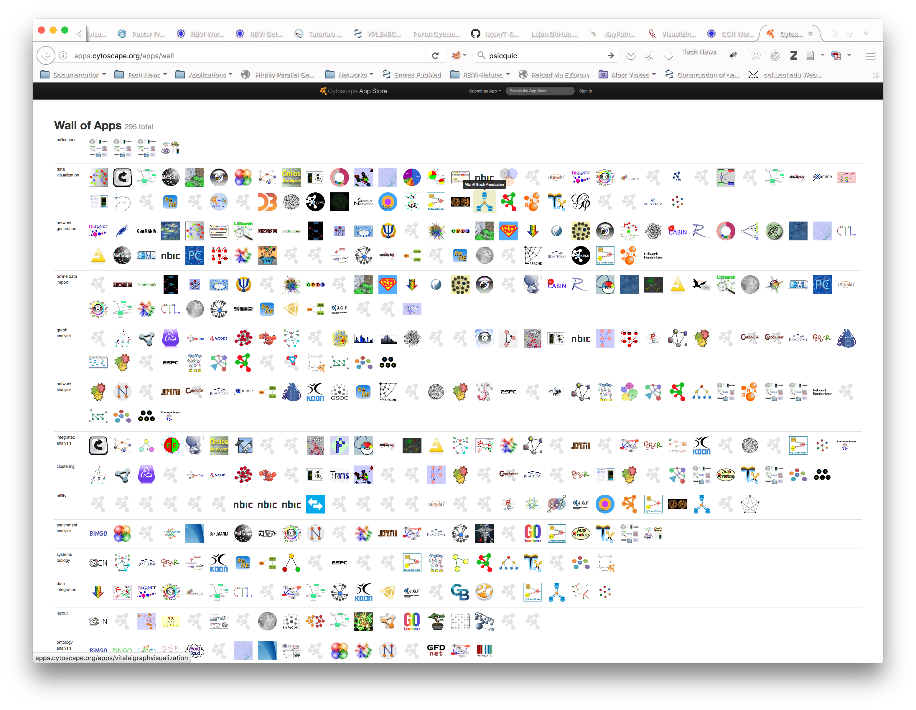
Figure 11.1: Available Cytoscape Apps
11.2.2 Overview of network biology themes and concepts
11.2.2.1 Why Networks?
Networks are everywhere…
- Molecular Networks
- Cell-Cell communication Networks
- Computer networks
- Social Networks
- Internet
Networks are powerful tools…
- Reduce complexity
- More efficient than tables
- Great for data integration
- Intuitive visualization
Often data in our pipelines are represented as data.frames, tables, matrices, vectors or lists. Sometimes we represent this data as heatmaps, or plots in efforts to summarize the results visually. Network visualization offers an additional method that readily incorporates many different data types and variables into a single picture.
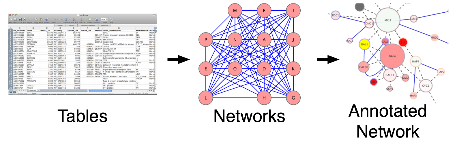
Figure 11.2: Translating data to networks
In order to translate your data into a network it is important to define the entities and their relationships. Entities and relationships can be anything. They can be user defined or they can be queried from a database.
Examples of Networks and their associated entities:
- Protein - Protein interaction network - is a directed or undirected network where nodes in the network are proteins or genes and edges represent how those proteins interact.
- Gene - gene interaction network - nodes in the network are genes and edges can represent synthetic lethality i.e. two genes have a connection if deleting both of them cause a decrease in fitness.
- Coexpression network - nodes in the network are genes or proteins and edges represent the degree of co-expression the two genes have. Often the edges are associated with a correlation score (i.e. pearson correlation) and edges are filtered by a defined threshold. If no threshold is specified all genes will be connected to all other genes creating a hairball.
- Enrichment Map - nodes in the networks are groups of genes from pathways or functions (i.e. genesets) and edges represent pathway crosstalk ( genes in common).
- Social network - nodes in the network are individuals and edges are some sort of social interaction between two individuals, for example, friends on Facebook, linked in LinkedIN, …
- Copublication network - a specialization of the social network for research purposes. Nodes in the network are individuals and edges between any two individuals for those who have co-authored a publication together.
11.2.3 Networks as Tools
Networks can be used for two main purposes but often go hand in hand.
Analysis
- Topological properties - including number of nodes, number of edges, node degree, average clustering coefficients, shortest path lengths, density, and many more. Topological properties can help gain insights into the structure and organization of the resulting biological networks as well as help highlight specific node or regions of the network.
- Hubs and subnetworks - a hub is generally a highly connected node in a scale-free network. Removal of hubs cause rapid breakdown of the underlying network. Subnetworks are interconnected regions of the network and can be defined by any user defined parameter.
- Cluster, classify, and diffuse
- Data integration
Visualization
- Data overlays
- Layouts and animation
- Exploratory analysis
- Context and interpretation
11.3 Translating biological data into Cytoscape using RCy3
Networks offer us a useful way to represent our biological data. But how do we seamlessly translate our data from R into Cytoscape?
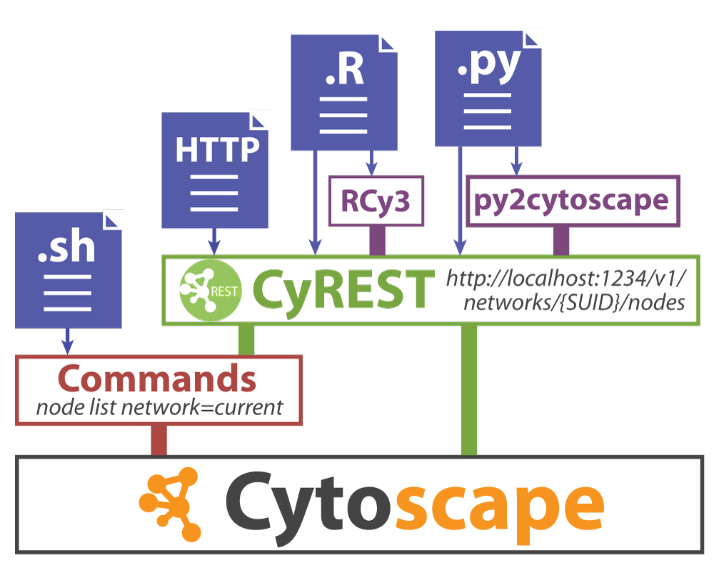
Figure 11.3: Different ways to communicate with Cytoscape
There are multiple ways to communicate with Cytoscape programmatically. There are two main complementary portals,cyRest(Ono et al. 2015) and Commands, that form the foundation. cyRest transforms Cytoscape in to a REST (Representational State Transfer) enabled service where it essentially listens for events through a predefined port (by default port 1234). The cyRest functionality started as an app add in but has now been incorporated into the main release. Commands, on the other hand, offer a mechanism whereby app developers can expose their functionality to other apps or to user through the command interface. Prior to the implementation of cyRest many of the basic network functions were first available as commands so there is some overlap between the two different methods. 11.3 shows the different ways you can call Cytoscape.
11.4 Set up
In order to create networks in Cytoscape from R you need:
- RCy3 - a biocondutor package
if(!"RCy3" %in% installed.packages()){
    install.packages("BiocManager")
    BiocManager::install("RCy3")
}
library(RCy3)- Cytoscape - Download and install Cytoscape 3.6.1. or higher. Java 9 in not supported. Please make sure that Java 8 is installed.
- Install additional cytoscape apps that will be used in this workshop. If using cytoscape 3.6.1 or older the apps need to manually installed through the app manager in Cytoscape or through your web browser. (click on the method to see detailed instructions)
- Functional Enrichment Collection -a collection of apps to retrieve networks and pathways, integrate and explore the data, perform functional enrichment analysis, and interpret and display your results.
- EnrichmentMap Pipeline Collection - a collection of apps including EnrichmentMap(Merico et al. 2010), AutoAnnotate(Kucera et al. 2016), WordCloud(Oesper et al. 2011) and clusterMaker2(Morris et al. 2011) used to visualize and analysis enrichment results.
If you are using Cytoscape 3.7 or higher (Cytoscape 3.7 will be released in August 2018) then apps can be installed directly from R.
#list of cytoscape apps to install
installation_responses <- c()

#list of app to install
cyto_app_toinstall <- c("clustermaker2", "enrichmentmap", "autoannotate", "wordcloud", "stringapp", "aMatReader")

cytoscape_version <- unlist(strsplit( cytoscapeVersionInfo()['cytoscapeVersion'],split = "\\."))
if(length(cytoscape_version) == 3 && as.numeric(cytoscape_version[1]>=3)
   && as.numeric(cytoscape_version[2]>=7)){
  for(i in 1:length(cyto_app_toinstall)){
    #check to see if the app is installed.  Only install it if it hasn't been installed
    if(!grep(commandsGET(paste("apps status app=\"", cyto_app_toinstall[i],"\"", sep="")),
             pattern = "status: Installed")){
      installation_response <-commandsGET(paste("apps install app=\"",
                                                cyto_app_toinstall[i],"\"", sep=""))
      installation_responses <- c(installation_responses,installation_response)
    } else{
      installation_responses <- c(installation_responses,"already installed")
    }
  }
  installation_summary <- data.frame(name = cyto_app_toinstall,
                                     status = installation_responses)

  knitr::kable(list(installation_summary),
  booktabs = TRUE, caption = 'A Summary of automated app installation'
)
}
Make sure that Cytoscape is open
cytoscapePing ()
11.4.1 Getting started
11.4.1.1 Confirm that Cytoscape is installed and opened
cytoscapeVersionInfo ()
11.4.1.2 Browse available functions, commands and arguments
Depending on what apps you have installed there is different functionality available.
To see all the functions available in RCy3 package
help(package=RCy3)Open swagger docs for live instances of CyREST API. The CyREST API list all the functions available in a base distribution of cytoscape. The below command will launch the swagger documentation in a web browser. Functions are clustered into categories. Expanding individual categories will show all the option available. Further expanding an individual command will show detailed documentation for the function, input, outputs and allow you to try and run the function. Running the function will show the url used for the query and all returned responses.
cyrestAPI() # CyREST APIAs mentioned above, there are two ways to interact with Cytoscape, through the Cyrest API or commands. To see the available commands in swagger similar to the Cyrest API.
commandsAPI() # Commands APITo get information about an individual command from the R environment you can also use the commandsHelp function. Simply specify what command you would like to get information on by adding its name to the command. For example “commandsHelp(”help string“)”
commandsHelp("help")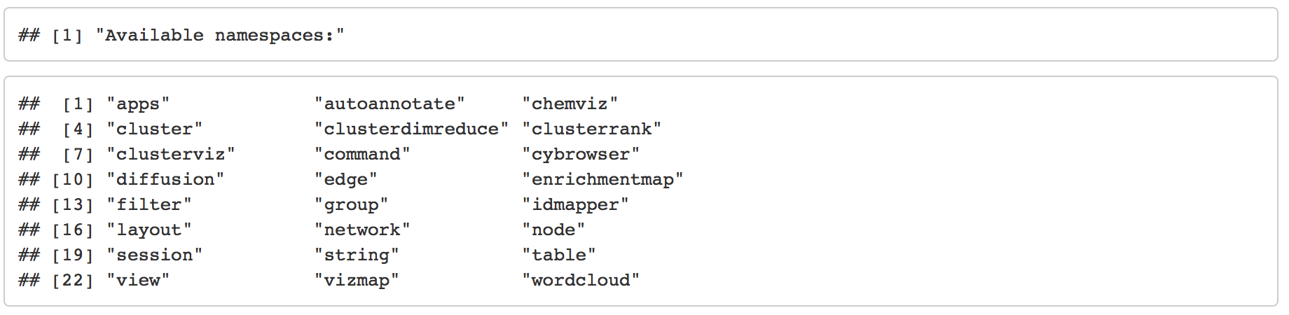
11.5 Cytoscape Basics
Create a Cytoscape network from some basic R objects
nodes <- data.frame(id=c("node 0","node 1","node 2","node 3"),
           group=c("A","A","B","B"), # categorical strings
           score=as.integer(c(20,10,15,5)), # integers
           stringsAsFactors=FALSE)
edges <- data.frame(source=c("node 0","node 0","node 0","node 2"),
           target=c("node 1","node 2","node 3","node 3"),
           interaction=c("inhibits","interacts","activates","interacts"),  # optional
           weight=c(5.1,3.0,5.2,9.9), # numeric
           stringsAsFactors=FALSE)
|
|
createNetworkFromDataFrames(nodes,edges, title="my first network", collection="DataFrame Example")
Remember. All networks we make are created in Cytoscape so get an image of the resulting network and include it in your current analysis if desired.
initial_network_png_file_name <- file.path(getwd(),"230_Isserlin_RCy3_intro", "images","initial_example_network.png")if(file.exists(initial_network_png_file_name)){
#cytoscape hangs waiting for user response if file already exists. Remove it first
file.remove(initial_network_png_file_name)
}
#export the network
exportImage(initial_network_png_file_name, type = "png")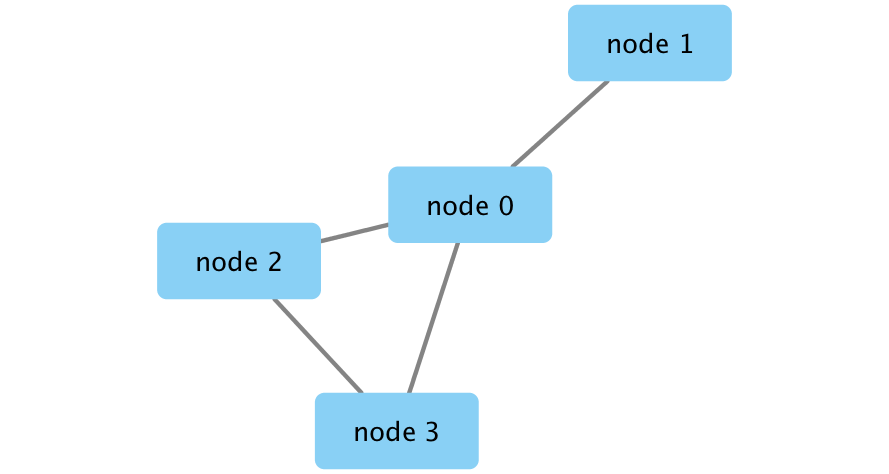
Figure 11.4: Example network created from dataframe
11.6 Example Data Set
We downloaded gene expression data from the Ovarian Serous Cystadenocarcinoma project of The Cancer Genome Atlas (TCGA)(International Cancer Genome et al. 2010), http://cancergenome.nih.gov via the Genomic Data Commons (GDC) portal(Grossman et al. 2016) on 2017-06-14 using TCGABiolinks R package(Colaprico et al. 2016). The data includes 300 samples available as RNA-seq data, with reads mapped to a reference genome using MapSplice(Wang et al. 2010) and read counts per transcript determined using the RSEM method(B. Li and Dewey 2011). RNA-seq data are labeled as ‘RNA-Seq V2’, see details at: https://wiki.nci.nih.gov/display/TCGA/RNASeq+Version+2). The RNA-SeqV2 data consists of raw counts similar to regular RNA-seq but RSEM (RNA-Seq by Expectation Maximization) data can be used with the edgeR method. The expression dataset of 300 tumours, with 79 classified as Immunoreactive, 72 classified as Mesenchymal, 69 classified as Differentiated, and 80 classified as Proliferative samples(class definitions were obtained from Verhaak et al.(Verhaak et al. 2013) Supplementary Table 1, third column). RNA-seq read counts were converted to CPM values and genes with CPM > 1 in at least 50 of the samples are retained for further study (50 is the minimal sample size in the classes). The data was normalized and differential expression was calculated for each cancer class relative to the rest of the samples.
There are two data files: 1. Expression matrix - containing the normalized expression for each gene across all 300 samples. 1. Gene ranks - containing the p-values, FDR and foldchange values for the 4 comparisons (mesenchymal vs rest, differential vs rest, proliferative vs rest and immunoreactive vs rest)
RNASeq_expression_matrix <- read.table(
  file.path(getwd(),"230_Isserlin_RCy3_intro","data","TCGA_OV_RNAseq_expression.txt"),
  header = TRUE, sep = "\t", quote="\"", stringsAsFactors = FALSE)

RNASeq_gene_scores <- read.table(
   file.path(getwd(),"230_Isserlin_RCy3_intro","data","TCGA_OV_RNAseq_All_edgeR_scores.txt"),
  header = TRUE, sep = "\t", quote="\"", stringsAsFactors = FALSE)
11.7 Finding Network Data
How do I represent my data as a network?
Unfortunately, there is not a simple answer. It depends on your biological question!
Example use cases:
- Omics data - I have a fill in the blank (microarray, RNASeq, Proteomics, ATACseq, MicroRNA, GWAS …) dataset. I have normalized and scored my data. How do I overlay my data on existing interaction data?
- Coexpression data - I have a dataset that represents relationships. How do I represent it as a network.
- Omics data - I have a fill in the blank (microarray, RNASeq, Proteomics, ATACseq, MicroRNA, GWAS …) dataset. I have normalized and scored my data. I have run my data through a functional enrichment tool and now have a set of enriched terms associated with my dataset. How do I represent my functional enrichments as a network?
11.8 Use Case 1 - How are my top genes related?
Omics data - I have a fill in the blank (microarray, RNASeq, Proteomics, ATACseq, MicroRNA, GWAS …) dataset. I have normalized and scored my data. How do I overlay my data on existing interaction data?
There are endless amounts of databases storing interaction data.
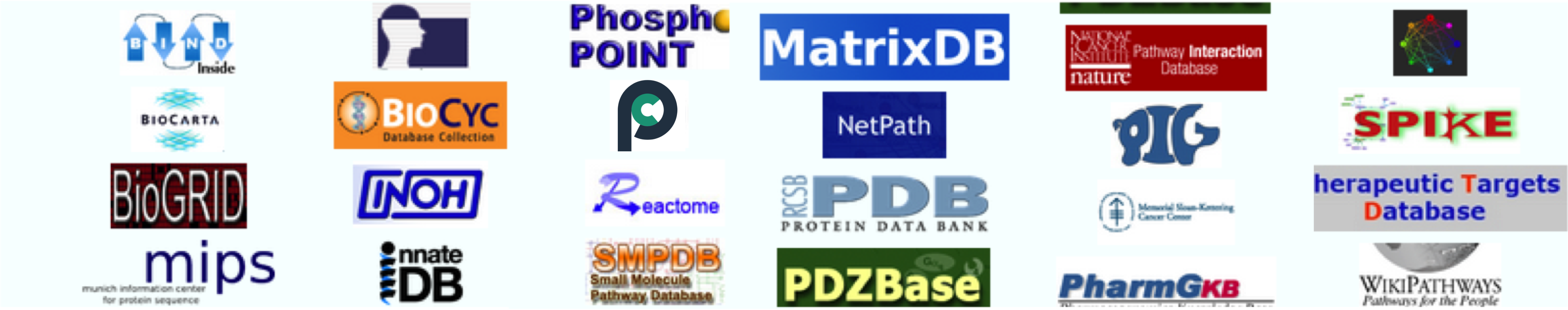
Figure 11.5: Info graphic of some of the available pathway databases
Thankfully we don’t have to query each independent ally. In addition to many specialized (for example, for specific molecules, interaction type, or species) interaction databases there are also databases that collate these databases to create a broad resource that is easier to use. For example:
- StringApp - is a protein - protein and protein- chemical database that imports data from String(Szklarczyk et al. 2016) (which itself includes data from multiple species, coexpression, text-mining,existing databases, and genomic context), [STITCH] into a unified, queriable database.
- PSICQUIC(Aranda et al. 2011) - a REST-ful service that is the responsibility of the database provider to set up and maintain. PSICQUIC is an additional interface that allows users to search all available databases (that support this REST-ful service). The databases are required to represent their interaction data in Proteomic Standards Initiative - molecular interaction (PSI-MI) format. To see a list of all the available data source see here
- nDex(Pratt et al. 2017) - a network data exchange repository.
- GeneMANIA(Mostafavi et al. 2008) - contains multiple networks (shared domains, physical interactions, pathways, predicted, co-expression, genetic interactions and co-localized network). Given a set of genes GeneMANIA selects and weights networks that optimize the connectivity between the query genes. GeneMANIA will also return additional genes that are highly related to your query set.
- PathwayCommons - (access the data through the CyPath2App) is a pathway and interaction data source. Data is collated from a large set of resources (list here ) and stored in the BioPAX(Demir et al. 2010) format. BioPAX is a data standard that allows for detailed representation of pathway mechanistic details as opposed to collapsing it to the set of interactions between molecules. BioPAX pathways from Pathway commons can also be loaded directly into R using the PaxToolsR(Luna et al. 2015) Bioconductor package.
Get a subset of genes of interest from our scored data:
top_mesenchymal_genes <- RNASeq_gene_scores[which(RNASeq_gene_scores$FDR.mesen < 0.05 & RNASeq_gene_scores$logFC.mesen > 2),]
head(top_mesenchymal_genes)
#>       Name geneid logFC.mesen logCPM.mesen  LR.mesen PValue.mesen
#> 188   PRG4  10216    2.705305    2.6139056  95.58179     1.42e-22
#> 252  PROK1  84432    2.543381    1.3255202  68.31067     1.40e-16
#> 308  PRRX1   5396    2.077538    4.8570983 123.09925     1.33e-28
#> 434  PTGFR   5737    2.075707   -0.1960881  73.24646     1.14e-17
#> 438  PTGIS   5740    2.094198    5.8279714 165.11038     8.65e-38
#> 1214 BARX1  56033    3.267472    1.7427387 166.30064     4.76e-38
#>      FDR.mesen logFC.diff logCPM.diff   LR.diff  PValue.diff     FDR.diff
#> 188   7.34e-21 -1.2716521   2.6139056 14.107056 1.726950e-04 1.181751e-03
#> 252   4.77e-15  0.7455119   1.3255202  5.105528 2.384972e-02 6.549953e-02
#> 308   1.08e-26 -1.2367108   4.8570983 29.949104 4.440000e-08 1.250000e-06
#> 434   4.30e-16 -0.4233297  -0.1960881  2.318523 1.278413e-01 2.368387e-01
#> 438   1.20e-35 -0.4448761   5.8279714  5.696086 1.700278e-02 5.027140e-02
#> 1214  6.82e-36 -2.4411370   1.7427387 52.224346 4.950000e-13 6.970000e-11
#>      Row.names.y logFC.immuno logCPM.immuno LR.immuno PValue.immuno
#> 188   PRG4|10216   -0.4980017     2.6139056  2.651951   0.103422901
#> 252  PROK1|84432   -1.9692994     1.3255202 27.876348   0.000000129
#> 308   PRRX1|5396   -0.4914091     4.8570983  5.773502   0.016269586
#> 434   PTGFR|5737   -0.6737143    -0.1960881  6.289647   0.012144523
#> 438   PTGIS|5740   -0.6138074     5.8279714 11.708780   0.000622059
#> 1214 BARX1|56033   -0.6063633     1.7427387  4.577141   0.032401228
#>       FDR.immuno logFC.prolif logCPM.prolif  LR.prolif PValue.prolif
#> 188  0.185548905   -0.9356510     2.6139056  8.9562066  0.0027652850
#> 252  0.000001650   -1.3195933     1.3255202 13.7675841  0.0002068750
#> 308  0.042062023   -0.3494185     4.8570983  2.9943819  0.0835537930
#> 434  0.033197211   -0.9786631    -0.1960881 12.9112727  0.0003266090
#> 438  0.002779895   -1.0355143     5.8279714 31.9162051  0.0000000161
#> 1214 0.073565295   -0.2199714     1.7427387  0.6315171  0.4267993850
#>       FDR.prolif
#> 188  0.006372597
#> 252  0.000622057
#> 308  0.128528698
#> 434  0.000932503
#> 438  0.000000107
#> 1214 0.510856262
We are going to query the String Database to get all interactions found for our set of top Mesenchymal genes.
Reminder: to see the parameters required by the string function or to find the right string function you can use commandsHelp.
commandsHelp("help string")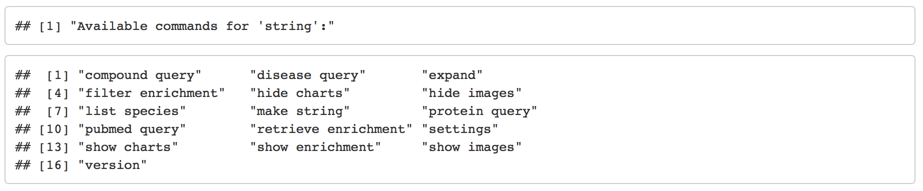
commandsHelp("help string protein query")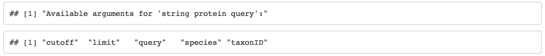
mesen_string_interaction_cmd <- paste('string protein query taxonID=9606 limit=150 cutoff=0.9 query="',paste(top_mesenchymal_genes$Name, collapse=","),'"',sep="")
commandsGET(mesen_string_interaction_cmd)
Get a screenshot of the initial network
initial_string_network_png_file_name <- file.path(getwd(),"230_Isserlin_RCy3_intro", "images", "initial_string_network.png")if(file.exists(initial_string_network_png_file_name)){
#cytoscape hangs waiting for user response if file already exists. Remove it first
response <- file.remove(initial_string_network_png_file_name)
}
response <- exportImage(initial_string_network_png_file_name, type = "png")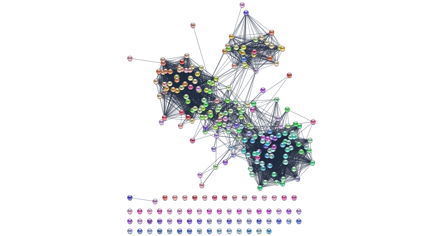
Figure 11.6: Initial network returned by String from our set of Mesenchymal query genes
Layout the network
layoutNetwork('force-directed')Check what other layout algorithms are available to try out
getLayoutNames()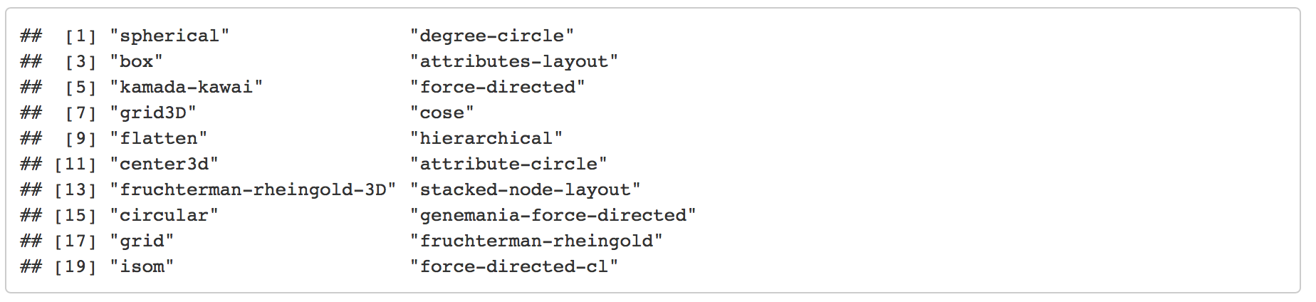 Get the parameters for a specific layout
getLayoutPropertyNames(layout.name='force-directed')
Re-layout the network using the force directed layout but specify some of the parameters
layoutNetwork('force-directed defaultSpringCoefficient=0.0000008 defaultSpringLength=70')Get a screenshot of the re-laid out network
relayout_string_network_png_file_name <- file.path(getwd(),"230_Isserlin_RCy3_intro", "images","relayout_string_network.png")if(file.exists(relayout_string_network_png_file_name)){
#cytoscape hangs waiting for user response if file already exists. Remove it first
response<- file.remove(relayout_string_network_png_file_name)
}
response <- exportImage(relayout_string_network_png_file_name, type = "png")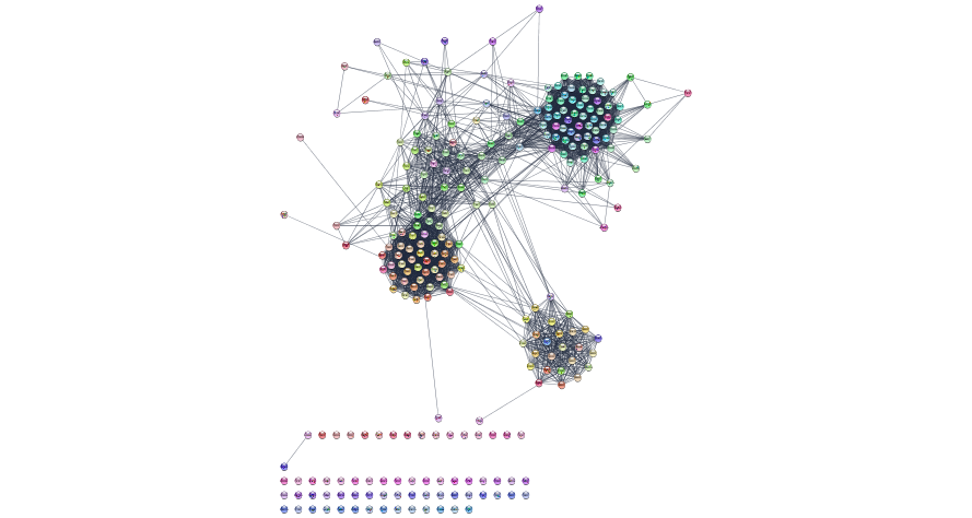
Figure 11.7: Initial network returned by String from our set of Mesenchymal query genes
Overlay our expression data on the String network.
To do this we will be using the loadTableData function from RCy3. It is important to make sure that that your identifiers types match up. You can check what is used by String by pulling in the column names of the node attribute table.
getTableColumnNames('node')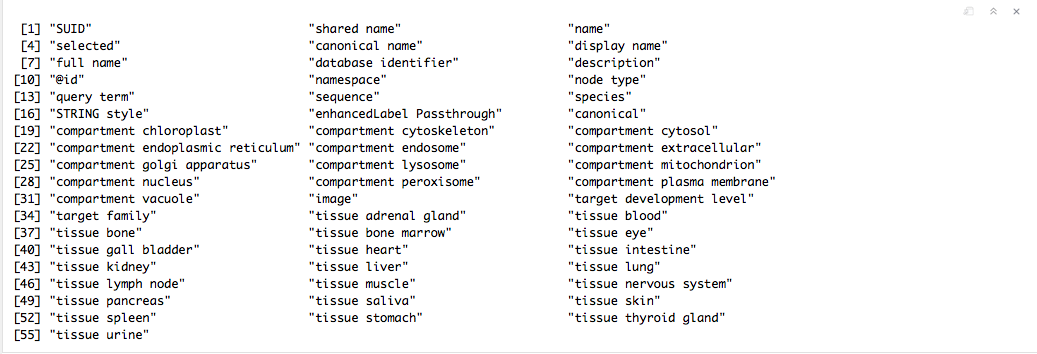
If you are unsure of what each column is and want to further verify the column to use you can also pull in the entire node attribute table.
node_attribute_table_topmesen <- getTableColumns(table="node")
head(node_attribute_table_topmesen[,3:7])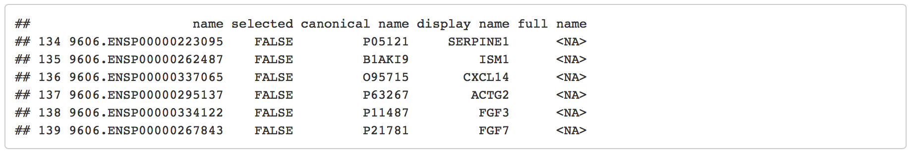
The column “display name” contains HGNC gene names which are also found in our Ovarian Cancer dataset.
To import our expression data we will match our dataset to the “display name” node attribute.
?loadTableData

loadTableData(RNASeq_gene_scores,table.key.column = "display name",data.key.column = "Name")  #default data.frame key is row.names
Modify the Visual Style Create your own visual style to visualize your expression data on the String network.
Start with a default style
style.name = "MesenchymalStyle"
defaults.list <- list(NODE_SHAPE="ellipse",
                 NODE_SIZE=60,
                 NODE_FILL_COLOR="#AAAAAA",
                 EDGE_TRANSPARENCY=120)
node.label.map <- mapVisualProperty('node label','display name','p') # p for passthrough; nothing else needed
createVisualStyle(style.name, defaults.list, list(node.label.map))
setVisualStyle(style.name=style.name)
Update your created style with a mapping for the Mesenchymal logFC expression. The first step is to grab the column data from Cytoscape (we can reuse the node_attribute table concept from above but we have to call the function again as we have since added our expression data) and pull out the min and max to define our data mapping range of values.
Note: you could define the min and max based on the entire dataset or just the subset that is represented in Cytoscape currently. The two methods will give you different results. If you intend on comparing different networks created with the same dataset then it is best to calculate the min and max from the entire dataset as opposed to a subset.
min.mesen.logfc = min(RNASeq_gene_scores$logFC.mesen,na.rm=TRUE)
max.mesen.logfc = max(RNASeq_gene_scores$logFC.mesen,na.rm=TRUE)
data.values = c(min.mesen.logfc,0,max.mesen.logfc)
Next, we use the RColorBrewer package to help us pick good colors to pair with our data values.
library(RColorBrewer)
display.brewer.all(length(data.values), colorblindFriendly=TRUE, type="div") # div,qual,seq,all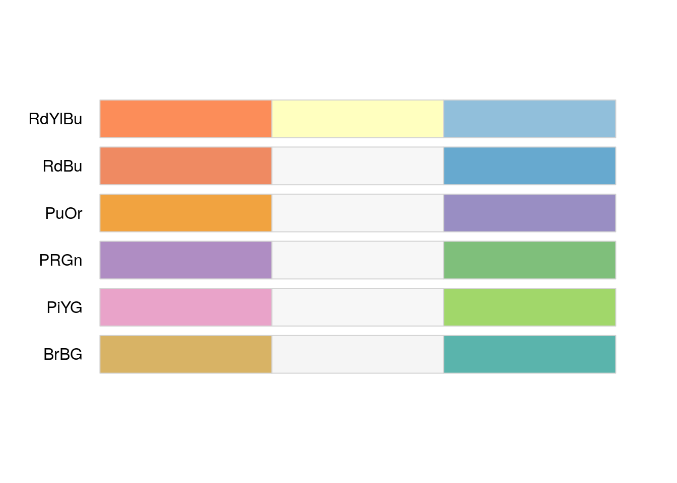
node.colors <- c(rev(brewer.pal(length(data.values), "RdBu")))Map the colors to our data value and update our visual style.
setNodeColorMapping("logFC.mesen", data.values, node.colors, style.name=style.name)Remember, String includes your query proteins as well as other proteins that associate with your query proteins (including the strongest connection first). Not all of the proteins in this network are your top hits. How can we visualize which proteins are our top Mesenchymal hits?
Add a different border color or change the node shape for our top hits.
getNodeShapes()

#select the Nodes of interest
#selectNode(nodes = top_mesenchymal_genes$Name, by.col="display name")
setNodeShapeBypass(node.names = top_mesenchymal_genes$Name, new.shapes = "TRIANGLE")
Change the size of the node to be correlated with the Mesenchymal p-value.
setNodeSizeMapping(table.column = 'LR.mesen',
                   table.column.values = c(min(RNASeq_gene_scores$LR.mesen),
                                           mean(RNASeq_gene_scores$LR.mesen),
                                           max(RNASeq_gene_scores$LR.mesen)),
                   sizes = c(30, 60, 150),mapping.type = "c", style.name = style.name)
Get a screenshot of the resulting network
mesen_string_network_png_file_name <- file.path(getwd(),"230_Isserlin_RCy3_intro", "images","mesen_string_network.png")if(file.exists(mesen_string_network_png_file_name)){
#cytoscape hangs waiting for user response if file already exists. Remove it first
response<- file.remove(mesen_string_network_png_file_name)
}
response <- exportImage(mesen_string_network_png_file_name, type = "png")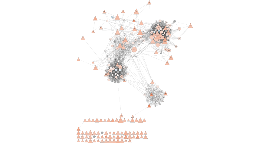
Figure 11.8: Formatted String network from our set of Mesenchymal query genes. Annotated with our expressin data
11.9 Use Case 2 - Which genes have similar expression.
Instead of querying existing resources look for correlations in your own dataset to find out which genes have similar expression. There are many tools that can analyze your data for correlation. A popular tool is Weighted Gene Correlation Network Analysis (WGCNA)(Langfelder and Horvath 2008) which takes expression data and calculates functional modules. As a simple example we can transform our expression dataset into a correlation matrix.
Using the Cytoscape App, aMatReader(Settle et al. 2018), we transform our adjacency matrix into an interaction network. First we filter the correlation matrix to contain only the strongest connections (for example, only correlations greater than 0.9).
RNASeq_expression <- RNASeq_expression_matrix[,3:ncol(RNASeq_expression_matrix)]

rownames(RNASeq_expression) <- RNASeq_expression_matrix$Name
RNAseq_correlation_matrix <- cor(t(RNASeq_expression), method="pearson")

#set the diagonal of matrix to zero - eliminate self-correlation
RNAseq_correlation_matrix[
  row(RNAseq_correlation_matrix) == col(RNAseq_correlation_matrix) ] <- 0

# set all correlations that are less than 0.9 to zero
RNAseq_correlation_matrix[which(RNAseq_correlation_matrix<0.90)] <- 0

#get rid of rows and columns that have no correlations with the above thresholds
RNAseq_correlation_matrix <- RNAseq_correlation_matrix[which(rowSums(RNAseq_correlation_matrix) != 0),
                          which(colSums(RNAseq_correlation_matrix) !=0)]

#write out the correlation file
correlation_filename <- file.path(getwd(), "230_Isserlin_RCy3_intro", "data", "TCGA_OV_RNAseq_expression_correlation_matrix.txt")
write.table( RNAseq_correlation_matrix,  file = correlation_filename, col.names  = TRUE, row.names = FALSE, sep = "\t", quote=FALSE)
Use the CyRest call to access the aMatReader functionality.
amat_url <- "aMatReader/v1/import"
amat_params = list(files = list(correlation_filename),
                   delimiter = "TAB",
                   undirected = FALSE,
                   ignoreZeros = TRUE,
                   interactionName = "correlated with",
                   rowNames = FALSE
                   )

response <- cyrestPOST(operation = amat_url, body = amat_params, base.url = "http://localhost:1234")

current_network_id <- response$data["suid"]
#relayout network
layoutNetwork('cose',
network = as.numeric(current_network_id))renameNetwork(title = "Coexpression_network_pear0_95",
network = as.numeric(current_network_id))Modify the visualization to see where each genes is predominantly expressed. Look at the 4 different p-values associated with each gene and color the nodes with the type associated with the lowest FDR.
Load in the scoring data. Specify the cancer type where the genes has the lowest FDR value.
nodes_in_network <- rownames(RNAseq_correlation_matrix)

#add an additional column to the gene scores table to indicate in which samples
# the gene is significant
node_class <- vector(length = length(nodes_in_network),mode = "character")
for(i in 1:length(nodes_in_network)){
  current_row <- which(RNASeq_gene_scores$Name == nodes_in_network[i])
  min_pvalue <- min(RNASeq_gene_scores[current_row,
                                       grep(colnames(RNASeq_gene_scores), pattern = "FDR")])
  if(RNASeq_gene_scores$FDR.mesen[current_row] <=min_pvalue){
    node_class[i] <- paste(node_class[i],"mesen",sep = " ")
  }
  if(RNASeq_gene_scores$FDR.diff[current_row] <=min_pvalue){
    node_class[i] <- paste(node_class[i],"diff",sep = " ")
  }
  if(RNASeq_gene_scores$FDR.prolif[current_row] <=min_pvalue){
    node_class[i] <- paste(node_class[i],"prolif",sep = " ")
  }
  if(RNASeq_gene_scores$FDR.immuno[current_row] <=min_pvalue){
    node_class[i] <- paste(node_class[i],"immuno",sep = " ")
  }
}
node_class <- trimws(node_class)
node_class_df <-data.frame(name=nodes_in_network, node_class,stringsAsFactors = FALSE)

head(node_class_df)
#>     name node_class
#> 1  ABCA6      mesen
#> 2  ABCA8      mesen
#> 3   ABI3     immuno
#> 4   ACAN     prolif
#> 5  ACAP1     immuno
#> 6 ADAM12      mesen
Map the new node attribute and the all the gene scores to the network.
loadTableData(RNASeq_gene_scores,table.key.column = "name",data.key.column = "Name")  #default data.frame key is row.names

loadTableData(node_class_df,table.key.column = "name",data.key.column = "name")  #default data.frame key is row.names
Create a color mapping for the different cancer types.
#create a new mapping with the different types
unique_types <- sort(unique(node_class))

coul = brewer.pal(4, "Set1")

# I can add more tones to this palette :
coul = colorRampPalette(coul)(length(unique_types))

setNodeColorMapping(table.column = "node_class",table.column.values = unique_types,
                    colors = coul,mapping.type = "d")
correlation_network_png_file_name <- file.path(getwd(),"230_Isserlin_RCy3_intro", "images","correlation_network.png")if(file.exists(correlation_network_png_file_name)){
#cytoscape hangs waiting for user response if file already exists. Remove it first
file.remove(correlation_network_png_file_name)
}
#export the network
exportImage(correlation_network_png_file_name, type = "png")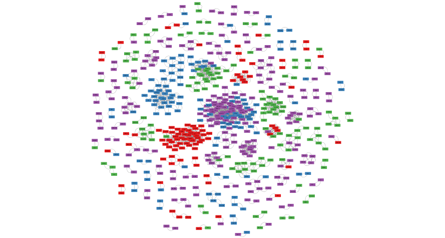
Figure 11.9: Example correlation network created using aMatReader
cluster the Network
#make sure it is set to the right network
  setCurrentNetwork(network = getNetworkName(suid=as.numeric(current_network_id)))

  #cluster the network
  clustermaker_url <- paste("cluster mcl network=SUID:",current_network_id, sep="")
  commandsGET(clustermaker_url)

  #get the clustering results
  default_node_table <- getTableColumns(table= "node",network = as.numeric(current_network_id))

  head(default_node_table)
Perform pathway Enrichment on one of the clusters using g:Profiler(Reimand et al. 2016). g:Profiler is an online functional enrichment web service that will take your gene list and return the set of enriched pathways. For automated analysis g:Profiler has created an R library to interact with it directly from R instead of using the web page.
Create a function to call g:Profiler and convert the returned results into a generic enrichment map input file.
tryCatch(expr = { library("gProfileR")},
         error = function(e) { install.packages("gProfileR")}, finally = library("gProfileR"))

#function to run gprofiler using the gprofiler library
#
# The function takes the returned gprofiler results and formats it to the generic EM input file
#
# function returns a data frame in the generic EM file format.
runGprofiler <- function(genes,current_organism = "hsapiens",
                         significant_only = F, set_size_max = 200,
                         set_size_min = 3, filter_gs_size_min = 5 , exclude_iea = F){

  gprofiler_results <- gprofiler(genes ,
                                 significant=significant_only,ordered_query = F,
                                exclude_iea=exclude_iea,max_set_size = set_size_max,
                                 min_set_size = set_size_min,
                                 correction_method = "fdr",
                                 organism = current_organism,
                                src_filter = c("GO:BP","REAC"))

  #filter results
  gprofiler_results <- gprofiler_results[which(gprofiler_results[,'term.size'] >= 3
                                        & gprofiler_results[,'overlap.size'] >= filter_gs_size_min ),]

  # gProfileR returns corrected p-values only.  Set p-value to corrected p-value
  if(dim(gprofiler_results)[1] > 0){
    em_results <- cbind(gprofiler_results[,
                                c("term.id","term.name","p.value","p.value")], 1,
                                gprofiler_results[,"intersection"])
  colnames(em_results) <- c("Name","Description", "pvalue","qvalue","phenotype","genes")

  return(em_results)
  } else {
    return("no gprofiler results for supplied query")
  }
}
Run g:Profiler. g:Profiler will return a set of pathways and functions that are found to be enriched in our query set of genes.
  current_cluster <- "1"
  #select all the nodes in cluster 1
  selectednodes <- selectNodes(current_cluster, by.col="__mclCluster")

  #create a subnetwork with cluster 1
  subnetwork_suid <- createSubnetwork(nodes="selected")

  renameNetwork("Cluster1_Subnetwork", network=as.numeric(subnetwork_suid))

  subnetwork_node_table <- getTableColumns(table= "node",network = as.numeric(subnetwork_suid))

  em_results <- runGprofiler(subnetwork_node_table$name)

 #write out the g:Profiler results
 em_results_filename <-file.path(getwd(),
                            "230_Isserlin_RCy3_intro", "data",paste("gprofiler_cluster",current_cluster,"enr_results.txt",sep="_"))

  write.table(em_results,em_results_filename,col.name=TRUE,sep="\t",row.names=FALSE,quote=FALSE)


  head(em_results)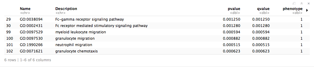
Create an enrichment map with the returned g:Profiler results. An enrichment map is a different sort of network. Instead of nodes representing genes, nodes represent pathways or functions. Edges between these pathways or functions represent shared genes or pathway crosstalk. An enrichment map is a way to visualize your enrichment results to help reduce redundancy and uncover main themes. Pathways can also be explored in detail using the features available through the App in Cytoscape.
 em_command = paste('enrichmentmap build analysisType="generic" ',
                   'pvalue=',"0.05", 'qvalue=',"0.05",
                   'similaritycutoff=',"0.25",
                   'coeffecients=',"JACCARD",
                   'enrichmentsDataset1=',em_results_filename ,
                   sep=" ")

  #enrichment map command will return the suid of newly created network.
  em_network_suid <- commandsRun(em_command)

  renameNetwork("Cluster1_enrichmentmap", network=as.numeric(em_network_suid))
Export image of resulting Enrichment map.
cluster1em_png_file_name <- file.path(getwd(),"230_Isserlin_RCy3_intro", "images","cluster1em.png")if(file.exists(cluster1em_png_file_name)){
#cytoscape hangs waiting for user response if file already exists. Remove it first
file.remove(cluster1em_png_file_name)
}
#export the network
exportImage(cluster1em_png_file_name, type = "png")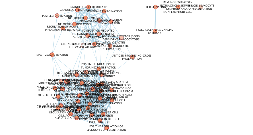
Figure 11.10: Example Enrichment Map created when running an enrichment analysis using g:Profiler with the genes that are part of cluster 1
Annotate the Enrichment map to get the general themes that are found in the enrichment results of cluster 1
#get the column from the nodetable and node table
  nodetable_colnames <- getTableColumnNames(table="node",  network =  as.numeric(em_network_suid))

  descr_attrib <- nodetable_colnames[grep(nodetable_colnames, pattern = "_GS_DESCR")]

  #Autoannotate the network
  autoannotate_url <- paste("autoannotate annotate-clusterBoosted labelColumn=", descr_attrib," maxWords=3 ", sep="")
    current_name <-commandsGET(autoannotate_url)
Export image of resulting Annotated Enrichment map.
cluster1em_annot_png_file_name <- file.path(getwd(),"230_Isserlin_RCy3_intro", "images","cluster1em_annot.png")if(file.exists(cluster1em_annot_png_file_name)){
#cytoscape hangs waiting for user response if file already exists. Remove it first
file.remove(cluster1em_annot_png_file_name)
}
#export the network
exportImage(cluster1em_annot_png_file_name, type = "png")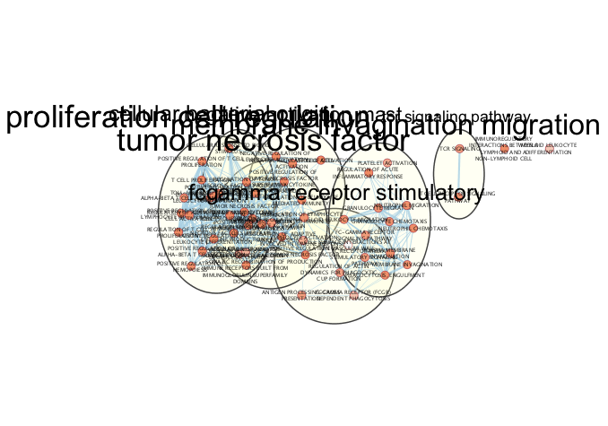
Figure 11.11: Example Annotated Enrichment Map created when running an enrichment analysis using g:Profiler with the genes that are part of cluster 1
Dense networks small or large never look like network figures we so often see in journals. A lot of manual tweaking, reorganization and optimization is involved in getting that perfect figure ready network. The above network is what the network starts as. The below figure is what it can look like after a few minutes of manual reorganiazation. (individual clusters were selected from the auto annotate panel and separated from other clusters)
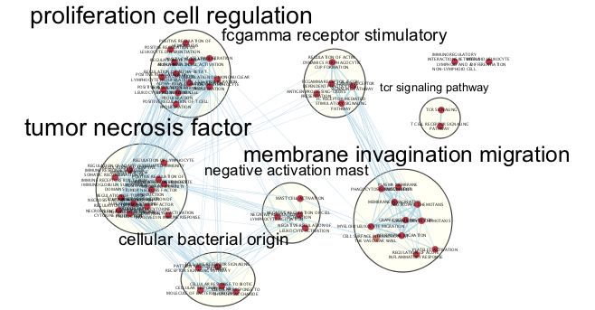
Figure 11.12: Example Annotated Enrichment Map created when running an enrichment analysis using g:Profiler with the genes that are part of cluster 1 after manual adjusting to generate a cleaner figure
11.10 Use Case 3 - Functional Enrichment of Omics set.
Reducing our large OMICs expression set to a simple list of genes eliminates the majority of the signals present in the data. Thresholding will only highlight the strong signals neglecting the often more interesting subtle signals. In order to capitalize on the wealth of data present in the data we need to perform pathway enrichment analysis on the entire expression set. There are many tools in R or as standalone apps that perform this type of analysis.
To demonstrate how you can use Cytoscape and RCy3 in your enrichment analysis pipeline we will use EnrichmentBrowser package (as demonstrated in detail in the workshop Functional enrichment analysis of high-throughput omics data) to perform pathway analysis.
if(!"EnrichmentBrowser" %in% installed.packages()){
    install.packages("BiocManager")
    BiocManager::install("EnrichmentBrowser")
}

suppressPackageStartupMessages(library(EnrichmentBrowser))
Download the latest pathway definition file from the Baderlab download site. Baderlab genesets are updated on a monthly basis. Detailed information about the sources can be found here. Only Human, Mouse and Rat gene set files are currently available on the Baderlab downloads site. If you are working with a species other than human (and it is either rat or mouse) change the gmt_url below to correct species.
tryCatch(expr = { suppressPackageStartupMessages(library("RCurl"))},
         error = function(e) {  install.packages("RCurl")},
         finally = library("RCurl"))

gmt_url = "http://download.baderlab.org/EM_Genesets/current_release/Human/symbol/"


#list all the files on the server
filenames = getURL(gmt_url)
tc = textConnection(filenames)
contents = suppressWarnings(readLines(tc))
close(tc)

#get the gmt that has all the pathways and does not include terms inferred from electronic annotations(IEA)
#start with gmt file that has pathways only
rx = gregexpr("(?<=<a href=\")(.*.GOBP_AllPathways_no_GO_iea.*.)(.gmt)(?=\">)",
  contents, perl = TRUE)
gmt_file = unlist(regmatches(contents, rx))

dest_gmt_file <- file.path(getwd(), "230_Isserlin_RCy3_intro", "data", gmt_file)

download.file(
    paste(gmt_url,gmt_file,sep=""),
    destfile=dest_gmt_file
)
Load in the gmt file
baderlab.gs <- getGenesets(dest_gmt_file)
baderlab.gs[1:2]
#> $`THIO-MOLYBDENUM COFACTOR BIOSYNTHESIS%HUMANCYC%PWY-5963`
#> [1] "MOCOS"
#>
#> $`PROLINE BIOSYNTHESIS I%HUMANCYC%PROSYN-PWY`
#> [1] "PYCR2"    "ALDH18A1" "PYCR1"    "PYCRL"
Create the dataset required by EnrichmentBrowser tools
#create the expression file - A tab separated text file containing expression values. Columns = samples/subjects; rows = features/probes/genes; NO headers, row or column names.
expr <- RNASeq_expression

sumexpr_filename <- file.path(getwd(), "230_Isserlin_RCy3_intro","data","SummarizeExperiment_expression.txt")
write.table( expr ,  file = sumexpr_filename , col.names  = FALSE, row.names = FALSE, sep = "\t", quote=FALSE)


rowData <- RNASeq_gene_scores[,grep(colnames(RNASeq_gene_scores), pattern="mesen")]
rowData <- cbind(RNASeq_gene_scores$Name,rowData)
colnames(rowData)[2] <- "FC"
colnames(rowData)[6] <- "ADJ.PVAL"

sumexpr_rdat_filename <- file.path(getwd(), "230_Isserlin_RCy3_intro","data","SummarizeExperiment_rdat.txt")
write.table( rowData[,1] ,  file = sumexpr_rdat_filename , col.names  = FALSE, row.names = FALSE, sep = "\t", quote=FALSE)

#load in the data classification data
# A tab separated text file containing annotation information for the samples in either *two or three* columns. NO headers, row or column names. The number of rows/samples in this file should match the number of columns/samples of the expression matrix. The 1st column is reserved for the sample IDs; The 2nd column is reserved for a *BINARY* group assignment. Use '0' and '1' for unaffected (controls) and affected (cases) sample class
classDefinitions_RNASeq <- read.table(
  file.path(getwd(), "230_Isserlin_RCy3_intro","data","RNASeq_classdefinitions.txt"), header = TRUE, sep = "\t", quote="\"", stringsAsFactors = FALSE)

colData <- data.frame(Sample = colnames(RNASeq_expression),
                      GROUP = classDefinitions_RNASeq$SUBTYPE,
                      stringsAsFactors = FALSE)
rownames(colData) <- colnames(RNASeq_expression)
colData$GROUP[which(colData$GROUP != "Mesenchymal")] <- 0
colData$GROUP[which(colData$GROUP == "Mesenchymal")] <- 1

sumexpr_cdat_filename <- file.path(getwd(), "230_Isserlin_RCy3_intro","data","SummarizeExperiment_cdat.txt")
write.table( colData ,  file = sumexpr_cdat_filename , col.names  = FALSE, row.names = FALSE, sep = "\t", quote=FALSE)

#create the Summarize Experiment object
se_OV <- EnrichmentBrowser::readSE(assay.file = sumexpr_filename , cdat.file = sumexpr_cdat_filename, rdat.file = sumexpr_rdat_filename)
Put our precomputed p-values and fold change values into the Summarized Experiment object so we can use our rankings for the analysis
#set the Summarized Experiment to our computed p-values and FC
rowData(se_OV) <- rowData
Run basic Over representation analysis (ORA) using our ranked genes and our gene set file downloaded from the Baderlab genesets.
ora.all <- sbea(method="ora", se=se_OV, gs=baderlab.gs, perm=0, alpha=0.05)
gsRanking(ora.all)
#> DataFrame with 967 rows and 4 columns
#>                                                                                            GENE.SET
#>                                                                                         <character>
#> 1                                                 EXTRACELLULAR MATRIX ORGANIZATION%GOBP%GO:0030198
#> 2   HALLMARK_EPITHELIAL_MESENCHYMAL_TRANSITION%MSIGDB_C2%HALLMARK_EPITHELIAL_MESENCHYMAL_TRANSITION
#> 3                                              EXTRACELLULAR STRUCTURE ORGANIZATION%GOBP%GO:0043062
#> 4                                        EXTRACELLULAR MATRIX ORGANIZATION%REACTOME%R-HSA-1474244.2
#> 5                                                 NABA_CORE_MATRISOME%MSIGDB_C2%NABA_CORE_MATRISOME
#> ...                                                                                             ...
#> 963                                                                 OVULATION CYCLE%GOBP%GO:0042698
#> 964                                                NEGATIVE REGULATION OF TRANSPORT%GOBP%GO:0051051
#> 965                                                  PEPTIDYL-TYROSINE MODIFICATION%GOBP%GO:0018212
#> 966                                                        NEUTROPHIL DEGRANULATION%GOBP%GO:0043312
#> 967           PROCESSING OF CAPPED INTRON-CONTAINING PRE-MRNA%REACTOME DATABASE ID RELEASE 65%72203
#>      NR.GENES NR.SIG.GENES   P.VALUE
#>     <numeric>    <numeric> <numeric>
#> 1         195          147  6.42e-21
#> 2         193          145  2.07e-20
#> 3         223          160  5.43e-19
#> 4         239          163   6.1e-16
#> 5         215          145  1.03e-13
#> ...       ...          ...       ...
#> 963        13            9    0.0487
#> 964       246          118    0.0488
#> 965        76           40     0.049
#> 966       416          194    0.0496
#> 967       213          103    0.0499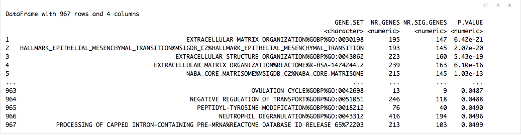
Take the enrichment results and create a generic enrichment map input file so we can create an Enrichment map. Description of format of the generic input file can be found here and example generic enrichment map files can be found here
#manually adjust p-values
ora.all$res.tbl <- cbind(ora.all$res.tbl, p.adjust(ora.all$res.tbl$P.VALUE, "BH"))
colnames(ora.all$res.tbl)[ncol(ora.all$res.tbl)] <- "Q.VALUE"

#create a generic enrichment map file
em_results_mesen <- data.frame(name = ora.all$res.tbl$GENE.SET,descr = ora.all$res.tbl$GENE.SET,
                               pvalue=ora.all$res.tbl$P.VALUE, qvalue=ora.all$res.tbl$Q.VALUE, stringsAsFactors = FALSE)

#write out the ora results
 em_results_mesen_filename <-file.path(getwd(),
                            "230_Isserlin_RCy3_intro","data","mesen_ora_enr_results.txt")

  write.table(em_results_mesen,em_results_mesen_filename,col.name=TRUE,sep="\t",row.names=FALSE,quote=FALSE)
Create an enrichment map with the returned ORA results.
 em_command = paste('enrichmentmap build analysisType="generic" ', "gmtFile=", dest_gmt_file,
                   'pvalue=',"0.05", 'qvalue=',"0.05",
                   'similaritycutoff=',"0.25",
                   'coeffecients=',"JACCARD",
                   'enrichmentsDataset1=',em_results_mesen_filename ,
                   sep=" ")

  #enrichment map command will return the suid of newly created network.
  em_mesen_network_suid <- commandsRun(em_command)

  renameNetwork("Mesenchymal_ORA_enrichmentmap", network=as.numeric(em_mesen_network_suid))
Export image of resulting Enrichment map.
mesenem_png_file_name <- file.path(getwd(),"230_Isserlin_RCy3_intro", "images","mesenem.png")if(file.exists(mesenem_png_file_name)){
#cytoscape hangs waiting for user response if file already exists. Remove it first
file.remove(mesenem_png_file_name)
}
#export the network
exportImage(mesenem_png_file_name, type = "png")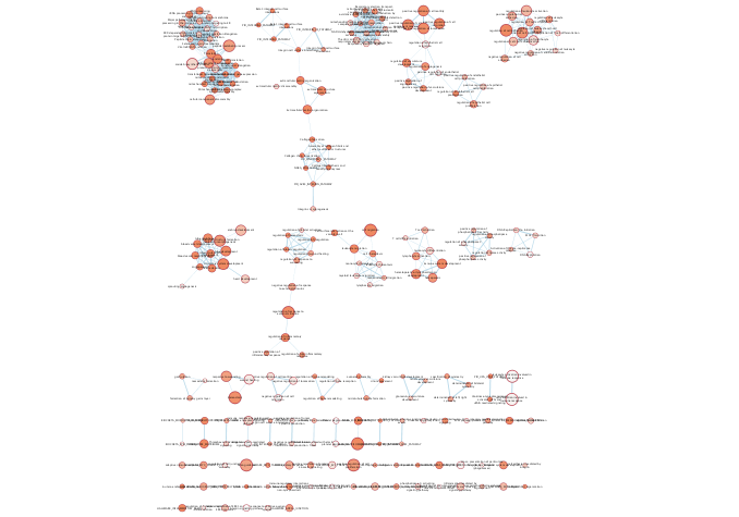
Figure 11.13: Example Enrichment Map created when running an enrichment analysis using EnrichmentBrowser ORA with the genes differential in Mesenchymal OV
Annotate the Enrichment map to get the general themes that are found in the enrichment results. Often for very busy networks annotating the networks doesn’t help to reduce the complexity but instead adds to it. To get rid of some of the pathway redundancy and density in the network create a summary of the underlying network. The summary network collapses each cluster to a summary node. Each summary node is annotated with a word tag (the top 3 words associated with the nodes of the cluster) that is computed using the Wordcloud app.
#get the column from the nodetable and node table
  nodetable_colnames <- getTableColumnNames(table="node",  network =  as.numeric(em_mesen_network_suid))

  descr_attrib <- nodetable_colnames[grep(nodetable_colnames, pattern = "_GS_DESCR")]

  #Autoannotate the network
  autoannotate_url <- paste("autoannotate annotate-clusterBoosted labelColumn=", descr_attrib," maxWords=3 ", sep="")
    current_name <-commandsGET(autoannotate_url)

  #create a summary network
  commandsGET("autoannotate summary network='current'")

  #change the network name
  summary_network_suid <- getNetworkSuid()

  renameNetwork(title = "Mesen_ORA_summary_netowrk",
              network = as.numeric(summary_network_suid))

  #get the summary node names
  summary_nodes <- getTableColumns(table="node",columns=c("name"))

  #clear bypass style the summary network has
  clearNodePropertyBypass(node.names = summary_nodes$name,visual.property = "NODE_SIZE")

  #relayout network
  layoutNetwork('cose',
              network = as.numeric(summary_network_suid))
Export image of resulting Summarized Annotated Enrichment map.
mesenem_summary_png_file_name <- file.path(getwd(),"230_Isserlin_RCy3_intro","images","mesenem_summary_network.png")if(file.exists(mesenem_summary_png_file_name)){
#cytoscape hangs waiting for user response if file already exists. Remove it first
file.remove(mesenem_summary_png_file_name)
}
#export the network
exportImage(mesenem_summary_png_file_name, type = "png")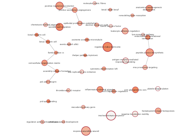
Figure 11.14: Example Annotated Enrichment Map created when running an enrichment analysis using EnrichmentBrowser ORA with the genes that differential in mesenchymal OV