The GenomicDataCommons Package
Sean Davis & Martin Morgan
Friday, February 07, 2025
Source:vignettes/overview.Rmd
overview.RmdAbstract
The National Cancer Institute (NCI) has established the Genomic Data Commons (GDC). The GDC provides the cancer research community with an open and unified repository for sharing and accessing data across numerous cancer studies and projects via a high-performance data transfer and query infrastructure. The GenomicDataCommons Bioconductor package provides basic infrastructure for querying, accessing, and mining genomic datasets available from the GDC. We expect that the Bioconductor developer and the larger bioinformatics communities will build on the GenomicDataCommons package to add higher-level functionality and expose cancer genomics data to the plethora of state-of-the-art bioinformatics methods available in Bioconductor.
What is the GDC?
From the Genomic Data Commons (GDC) website:
The National Cancer Institute’s (NCI’s) Genomic Data Commons (GDC) is a data sharing platform that promotes precision medicine in oncology. It is not just a database or a tool; it is an expandable knowledge network supporting the import and standardization of genomic and clinical data from cancer research programs. The GDC contains NCI-generated data from some of the largest and most comprehensive cancer genomic datasets, including The Cancer Genome Atlas (TCGA) and Therapeutically Applicable Research to Generate Effective Therapies (TARGET). For the first time, these datasets have been harmonized using a common set of bioinformatics pipelines, so that the data can be directly compared. As a growing knowledge system for cancer, the GDC also enables researchers to submit data, and harmonizes these data for import into the GDC. As more researchers add clinical and genomic data to the GDC, it will become an even more powerful tool for making discoveries about the molecular basis of cancer that may lead to better care for patients.
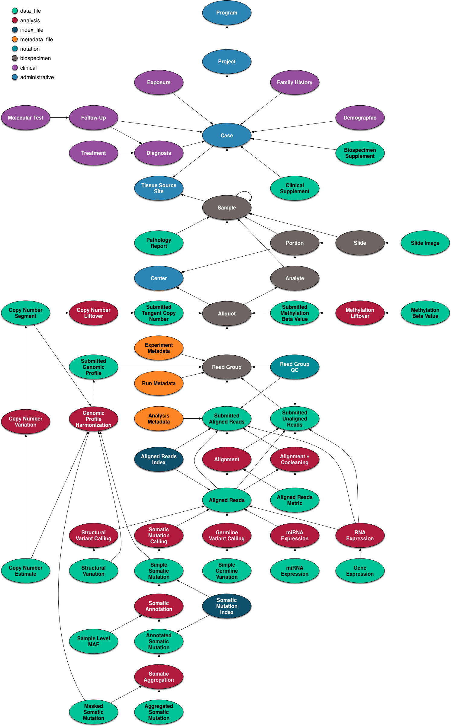
The data model for the GDC is complex, but it worth a quick overview and a graphical representation is included here.
The GDC API exposes these nodes and edges in a somewhat simplified set of RESTful endpoints.
Quickstart
This quickstart section is just meant to show basic functionality. More details of functionality are included further on in this vignette and in function-specific help.
This software is available at Bioconductor.org and can be downloaded
via BiocManager::install.
To report bugs or problems, either submit
a new issue or submit a
bug.report(package='GenomicDataCommons') from within R
(which will redirect you to the new issue on GitHub).
Installation
Installation can be achieved via Bioconductor’s
BiocManager package.
if (!require("BiocManager"))
    install.packages("BiocManager")
BiocManager::install('GenomicDataCommons')Check connectivity and status
The GenomicDataCommons
package relies on having network connectivity. In addition, the NCI GDC
API must also be operational and not under maintenance. Checking
status can be used to check this connectivity and
functionality.
GenomicDataCommons::status()## $commit
## [1] "48add4be7ac46e7db10e0c6f0e3010d5bb2a50aa"
##
## $data_release
## [1] "Data Release 42.0 - January 30, 2025"
##
## $data_release_version
## $data_release_version$major
## [1] 42
##
## $data_release_version$minor
## [1] 0
##
## $data_release_version$release_date
## [1] "2025-01-30"
##
##
## $status
## [1] "OK"
##
## $tag
## [1] "7.7"
##
## $version
## [1] 1And to check the status in code:
Find data
The following code builds a manifest that can be used to
guide the download of raw data. Here, filtering finds gene expression
files quantified as raw counts using STAR from ovarian
cancer patients.
ge_manifest <- files() |>
    filter( cases.project.project_id == 'TCGA-OV') |>
    filter( type == 'gene_expression' ) |>
    filter( analysis.workflow_type == 'STAR - Counts')  |>
    manifest()
head(ge_manifest)
## # A tibble: 6 × 17
## id data_format access file_name submitter_id data_category acl_1 type
## <chr> <chr> <chr> <chr> <chr> <chr> <chr> <chr>
## 1 46820e4f-… TSV contr… d6472bd0… 8a0bcacd-f0… Transcriptom… phs0… gene…
## 2 ab6ec803-… TSV contr… a14ac53b… b29ecf07-51… Transcriptom… phs0… gene…
## 3 04ab577f-… TSV open b6bc859c… 8ad5987b-1e… Transcriptom… open gene…
## 4 0f72e97c-… TSV open 517eb355… 284d7f95-ee… Transcriptom… open gene…
## 5 e20a8bed-… TSV contr… 676462aa… 00007463-be… Transcriptom… phs0… gene…
## 6 c33cb0b7-… TSV open dfe1fbdb… e7765e2f-59… Transcriptom… open gene…
## # ℹ 9 more variables: platform <chr>, file_size <int>, created_datetime <chr>,
## # md5sum <chr>, updated_datetime <chr>, file_id <chr>, data_type <chr>,
## # state <chr>, experimental_strategy <chr>Download data
After the 858 gene expression files specified in the query above.
Using multiple processes to do the download very significantly speeds up
the transfer in many cases. On a standard 1Gb connection, the following
completes in about 30 seconds. The first time the data are downloaded, R
will ask to create a cache directory (see ?gdc_cache for
details of setting and interacting with the cache). Resulting downloaded
files will be stored in the cache directory. Future access to the same
files will be directly from the cache, alleviating multiple
downloads.
fnames <- lapply(ge_manifest$id[1:20], gdcdata)If the download had included controlled-access data, the download
above would have needed to include a token. Details are
available in the authentication section
below.
Metadata queries
Clinical data
Accessing clinical data is a very common task. Given a set of
case_ids, the gdc_clinical() function will
return a list of four tibbles.
- demographic
- diagnoses
- exposures
- main
case_ids = cases() |> results(size=10) |> ids()
clindat = gdc_clinical(case_ids)
names(clindat)## [1] "demographic" "diagnoses" "exposures" "follow_ups" "main"
head(clindat[["main"]])## # A tibble: 6 × 13
## id lost_to_followup days_to_lost_to_foll…¹ created_datetime
## <chr> <chr> <lgl> <chr>
## 1 69eced5b-1e76-45c9-b… NA NA 2018-10-02T15:5…
## 2 e3b32485-b204-43a7-9… NA NA 2019-02-19T09:2…
## 3 4829dd8c-5445-41b3-a… NA NA 2020-07-31T09:2…
## 4 d420e653-3fb2-432b-9… NA NA 2019-10-14T10:4…
## 5 bfe15f44-e1dd-46ed-b… NA NA 2019-08-14T15:1…
## 6 8b3b1f24-419e-4043-8… NA NA 2018-10-02T15:5…
## # ℹ abbreviated name: ¹days_to_lost_to_followup
## # ℹ 9 more variables: updated_datetime <chr>, case_id <chr>, state <chr>,
## # disease_type <chr>, submitter_id <chr>, primary_site <chr>,
## # index_date <chr>, days_to_consent <lgl>, consent_type <lgl>
head(clindat[["diagnoses"]])## # A tibble: 6 × 10⁸
## case_id irs_stage iss_stage ajcc_pathologic_stage ann_arbor_clinical_s…¹
## <chr> <lgl> <lgl> <chr> <lgl>
## 1 69eced5b-1e7… NA NA NA NA
## 2 e3b32485-b20… NA NA Stage III NA
## 3 4829dd8c-544… NA NA NA NA
## 4 d420e653-3fb… NA NA NA NA
## 5 bfe15f44-e1d… NA NA Stage I NA
## 6 8b3b1f24-419… NA NA Stage I NA
## # ℹ abbreviated name: ¹ann_arbor_clinical_stage
## # ℹ 103 more variables: created_datetime <dttm>, enneking_msts_stage <lgl>,
## # inrg_stage <lgl>, enneking_msts_metastasis <lgl>,
## # tissue_or_organ_of_origin <chr>, age_at_diagnosis <int>,
## # esophageal_columnar_dysplasia_degree <lgl>, cog_liver_stage <lgl>,
## # child_pugh_classification <lgl>, metastasis_at_diagnosis_site <lgl>,
## # state <chr>, prior_treatment <chr>, …General metadata queries
The GenomicDataCommons
package can access the significant clinical, demographic, biospecimen,
and annotation information contained in the NCI GDC. The
gdc_clinical() function will often be all that is needed,
but the API and GenomicDataCommons
package make much flexibility if fine-tuning is required.
expands = c("diagnoses","annotations",
"demographic","exposures")
clinResults = cases() |>
GenomicDataCommons::select(NULL) |>
GenomicDataCommons::expand(expands) |>
results(size=50)
str(clinResults[[1]],list.len=6)## chr [1:50] "69eced5b-1e76-45c9-bc9c-2aa71a921c57" ...
# or listviewer::jsonedit(clinResults)Basic design
This package design is meant to have some similarities to the “hadleyverse” approach of dplyr. Roughly, the functionality for finding and accessing files and metadata can be divided into:
- Simple query constructors based on GDC API endpoints.
- A set of verbs that when applied, adjust filtering, field selection, and faceting (fields for aggregation) and result in a new query object (an endomorphism)
- A set of verbs that take a query and return results from the GDC
In addition, there are exhiliary functions for asking the GDC API for information about available and default fields, slicing BAM files, and downloading actual data files. Here is an overview of functionality1.
- Creating a query
- Manipulating a query
- Introspection on the GDC API fields
- Executing an API call to retrieve query results
- Raw data file downloads
- Summarizing and aggregating field values (faceting)
- Authentication
- BAM file slicing
Usage
There are two main classes of operations when working with the NCI GDC.
- Querying metadata and finding data files (e.g., finding all gene expression quantifications data files for all colon cancer patients).
- Transferring raw or processed data from the GDC to another computer (e.g., downloading raw or processed data)
Both classes of operation are reviewed in detail in the following sections.
Querying metadata
Vast amounts of metadata about cases (patients, basically), files,
projects, and so-called annotations are available via the NCI GDC API.
Typically, one will want to query metadata to either focus in on a set
of files for download or transfer or to perform so-called
aggregations (pivot-tables, facets, similar to the R
table() functionality).
Querying metadata starts with creating a
“blank” query. One will often then want to filter the query to limit results
prior to retrieving results. The
GenomicDataCommons package has helper
functions for listing fields that are available for filtering.
In addition to fetching results, the GDC API allows faceting, or aggregating,, useful for compiling reports, generating dashboards, or building user interfaces to GDC data (see GDC web query interface for a non-R-based example).
Creating a query
A query of the GDC starts its life in R. Queries follow the four
metadata endpoints available at the GDC. In particular, there are four
convenience functions that each create GDCQuery objects
(actually, specific subclasses of GDCQuery):
pquery = projects()The pquery object is now an object of (S3) class,
GDCQuery (and gdc_projects and
list). The object contains the following elements:
- fields: This is a character vector of the fields that will be
returned when we retrieve data. If no
fields are specified to, for example, the
projects()function, the default fields from the GDC are used (seedefault_fields()) - filters: This will contain results after calling the
filter()method and will be used to filter results on retrieval. - facets: A character vector of field names that will be used for aggregating data in a call to
aggregations(). - token: A character(1) token from the GDC. See the authentication section for details, but note that, in general, the token is not necessary for metadata query and retrieval, only for actual data download.
Looking at the actual object (get used to using str()!),
note that the query contains no results.
str(pquery)## List of 4
## $ fields : chr [1:10] "dbgap_accession_number" "disease_type" "intended_release_date" "name" ...
## $ filters: NULL
## $ facets : NULL
## $ expand : NULL
## - attr(*, "class")= chr [1:3] "gdc_projects" "GDCQuery" "list"Retrieving results
[ GDC pagination documentation ]
With a query object available, the next step is to retrieve results
from the GDC. The GenomicDataCommons package. The most basic type of
results we can get is a simple count() of records available
that satisfy the filter criteria. Note that we have not set any filters,
so a count() here will represent all the project records
publicly available at the GDC in the “default” archive”
## [1] 86The results() method will fetch actual results.
presults = pquery |> results()These results are returned from the GDC in JSON format and converted into a
(potentially nested) list in R. The str() method is useful
for taking a quick glimpse of the data.
str(presults)## List of 9
## $ id : chr [1:10] "HCMI-CMDC" "TCGA-KIRC" "CTSP-DLBCL1" "TCGA-BRCA" ...
## $ primary_site :List of 10
## ..$ HCMI-CMDC : chr [1:24] "Stomach" "Uterus, NOS" "Connective, subcutaneous and other soft tissues" "Skin" ...
## ..$ TCGA-KIRC : chr "Kidney"
## ..$ CTSP-DLBCL1: chr [1:2] "Unknown" "Lymph nodes"
## ..$ TCGA-BRCA : chr "Breast"
## ..$ MP2PRT-WT : chr "Kidney"
## ..$ CPTAC-3 : chr [1:10] "Bronchus and lung" "Breast" "Uterus, NOS" "Other and ill-defined sites" ...
## ..$ MATCH-P : chr [1:15] "Colon" "Small intestine" "Anus and anal canal" "Bladder" ...
## ..$ MATCH-W : chr [1:18] "Prostate gland" "Rectum" "Anus and anal canal" "Bladder" ...
## ..$ MATCH-Z1D : chr [1:15] "Small intestine" "Prostate gland" "Thyroid gland" "Other and unspecified female genital organs" ...
## ..$ MATCH-Z1A : chr [1:14] "Colon" "Rectum" "Ovary" "Bladder" ...
## $ dbgap_accession_number: chr [1:10] NA NA "phs001184" NA ...
## $ project_id : chr [1:10] "HCMI-CMDC" "TCGA-KIRC" "CTSP-DLBCL1" "TCGA-BRCA" ...
## $ disease_type :List of 10
## ..$ HCMI-CMDC : chr [1:16] "Soft Tissue Tumors and Sarcomas, NOS" "Complex Mixed and Stromal Neoplasms" "Acinar Cell Neoplasms" "Squamous Cell Neoplasms" ...
## ..$ TCGA-KIRC : chr "Adenomas and Adenocarcinomas"
## ..$ CTSP-DLBCL1: chr "Mature B-Cell Lymphomas"
## ..$ TCGA-BRCA : chr [1:9] "Epithelial Neoplasms, NOS" "Adnexal and Skin Appendage Neoplasms" "Squamous Cell Neoplasms" "Adenomas and Adenocarcinomas" ...
## ..$ MP2PRT-WT : chr "Neoplasms, NOS"
## ..$ CPTAC-3 : chr [1:11] "Squamous Cell Neoplasms" "Gliomas" "Adenomas and Adenocarcinomas" "Epithelial Neoplasms, NOS" ...
## ..$ MATCH-P : chr [1:10] "Transitional Cell Papillomas and Carcinomas" "Complex Mixed and Stromal Neoplasms" "Mesothelial Neoplasms" "Ductal and Lobular Neoplasms" ...
## ..$ MATCH-W : chr [1:8] "Adenomas and Adenocarcinomas" "Ductal and Lobular Neoplasms" "Epithelial Neoplasms, NOS" "Neoplasms, NOS" ...
## ..$ MATCH-Z1D : chr [1:8] "Complex Mixed and Stromal Neoplasms" "Myomatous Neoplasms" "Ductal and Lobular Neoplasms" "Neoplasms, NOS" ...
## ..$ MATCH-Z1A : chr [1:6] "Adenomas and Adenocarcinomas" "Mesothelial Neoplasms" "Epithelial Neoplasms, NOS" "Neoplasms, NOS" ...
## $ name : chr [1:10] "NCI Cancer Model Development for the Human Cancer Model Initiative" "Kidney Renal Clear Cell Carcinoma" "CTSP Diffuse Large B-Cell Lymphoma (DLBCL) CALGB 50303" "Breast Invasive Carcinoma" ...
## $ releasable : logi [1:10] TRUE TRUE TRUE TRUE FALSE TRUE ...
## $ state : chr [1:10] "open" "open" "open" "open" ...
## $ released : logi [1:10] TRUE TRUE TRUE TRUE TRUE TRUE ...
## - attr(*, "row.names")= int [1:10] 1 2 3 4 5 6 7 8 9 10
## - attr(*, "class")= chr [1:3] "GDCprojectsResults" "GDCResults" "list"A default of only 10 records are returned. We can use the
size and from arguments to
results() to either page through results or to change the
number of results. Finally, there is a convenience method,
results_all() that will simply fetch all the available
results given a query. Note that results_all() may take a
long time and return HUGE result sets if not used carefully. Use of a
combination of count() and results() to get a
sense of the expected data size is probably warranted before calling
results_all()
## [1] 10
presults = pquery |> results_all()
length(ids(presults))## [1] 86## [1] TRUEExtracting subsets of results or manipulating the results into a more conventional R data structure is not easily generalizable. However, the purrr, rlist, and data.tree packages are all potentially of interest for manipulating complex, nested list structures. For viewing the results in an interactive viewer, consider the listviewer package.
Fields and Values
Central to querying and retrieving data from the GDC is the ability
to specify which fields to return, filtering by fields and values, and
faceting or aggregating. The GenomicDataCommons package includes two
simple functions, available_fields() and
default_fields(). Each can operate on a character(1)
endpoint name (“cases”, “files”, “annotations”, or “projects”) or a
GDCQuery object.
default_fields('files')## [1] "access" "acl"
## [3] "average_base_quality" "average_insert_size"
## [5] "average_read_length" "cancer_dna_fraction"
## [7] "channel" "chip_id"
## [9] "chip_position" "contamination"
## [11] "contamination_error" "created_datetime"
## [13] "data_category" "data_format"
## [15] "data_type" "error_type"
## [17] "experimental_strategy" "file_autocomplete"
## [19] "file_id" "file_name"
## [21] "file_size" "genome_doubling"
## [23] "imaging_date" "magnification"
## [25] "md5sum" "mean_coverage"
## [27] "msi_score" "msi_status"
## [29] "pairs_on_diff_chr" "plate_name"
## [31] "plate_well" "platform"
## [33] "proc_internal" "proportion_base_mismatch"
## [35] "proportion_coverage_10x" "proportion_coverage_30x"
## [37] "proportion_reads_duplicated" "proportion_reads_mapped"
## [39] "proportion_targets_no_coverage" "read_pair_number"
## [41] "revision" "stain_type"
## [43] "state" "state_comment"
## [45] "subclonal_genome_fraction" "submitter_id"
## [47] "tags" "total_reads"
## [49] "tumor_ploidy" "tumor_purity"
## [51] "type" "updated_datetime"
## [53] "wgs_coverage"
# The number of fields available for files endpoint
length(available_fields('files'))## [1] 1193
# The first few fields available for files endpoint
head(available_fields('files'))## [1] "access" "acl"
## [3] "analysis.analysis_id" "analysis.analysis_type"
## [5] "analysis.created_datetime" "analysis.input_files.access"The fields to be returned by a query can be specified following a
similar paradigm to that of the dplyr package. The select()
function is a verb that resets the fields slot of a
GDCQuery; note that this is not quite analogous to the
dplyr select() verb that limits from already-present
fields. We completely replace the fields when using
select() on a GDCQuery.
# Default fields here
qcases = cases()
qcases$fields## [1] "aliquot_ids" "analyte_ids"
## [3] "case_autocomplete" "case_id"
## [5] "consent_type" "created_datetime"
## [7] "days_to_consent" "days_to_lost_to_followup"
## [9] "diagnosis_ids" "disease_type"
## [11] "index_date" "lost_to_followup"
## [13] "portion_ids" "primary_site"
## [15] "sample_ids" "slide_ids"
## [17] "state" "submitter_aliquot_ids"
## [19] "submitter_analyte_ids" "submitter_diagnosis_ids"
## [21] "submitter_id" "submitter_portion_ids"
## [23] "submitter_sample_ids" "submitter_slide_ids"
## [25] "updated_datetime"
# set up query to use ALL available fields
# Note that checking of fields is done by select()
qcases = cases() |> GenomicDataCommons::select(available_fields('cases'))
head(qcases$fields)## [1] "case_id" "aliquot_ids"
## [3] "analyte_ids" "annotations.annotation_id"
## [5] "annotations.case_id" "annotations.case_submitter_id"Finding fields of interest is such a common operation that the
GenomicDataCommons includes the grep_fields() function. See
the appropriate help pages for details.
Facets and aggregation
The GDC API offers a feature known as aggregation or faceting. By
specifying one or more fields (of appropriate type), the GDC can return
to us a count of the number of records matching each potential value.
This is similar to the R table method. Multiple fields can
be returned at once, but the GDC API does not have a cross-tabulation
feature; all aggregations are only on one field at a time. Results of
aggregation() calls come back as a list of data.frames
(actually, tibbles).
# total number of files of a specific type
res = files() |> facet(c('type','data_type')) |> aggregations()
res$type## doc_count key
## 1 196351 annotated_somatic_mutation
## 2 174046 aligned_reads
## 3 136937 structural_variation
## 4 127458 simple_somatic_mutation
## 5 89858 copy_number_segment
## 6 51028 gene_expression
## 7 39593 aggregated_somatic_mutation
## 8 39002 copy_number_estimate
## 9 36556 mirna_expression
## 10 33476 slide_image
## 11 33146 masked_methylation_array
## 12 27344 biospecimen_supplement
## 13 24236 submitted_genotyping_array
## 14 23135 simple_germline_variation
## 15 21589 masked_somatic_mutation
## 16 16573 methylation_beta_value
## 17 16273 copy_number_auxiliary_file
## 18 14427 clinical_supplement
## 19 11324 pathology_report
## 20 7906 protein_expression
## 21 1426 submitted_expression_array
## 22 132 secondary_expression_analysisUsing aggregations() is an also easy way to learn the
contents of individual fields and forms the basis for faceted search
pages.
Filtering
[
GDC filtering documentation ]
The GenomicDataCommons package uses a form of non-standard evaluation to specify R-like queries that are then translated into an R list. That R list is, upon calling a method that fetches results from the GDC API, translated into the appropriate JSON string. The R expression uses the formula interface as suggested by Hadley Wickham in his vignette on non-standard evaluation
It’s best to use a formula because a formula captures both the expression to evaluate and the environment where the evaluation occurs. This is important if the expression is a mixture of variables in a data frame and objects in the local environment [for example].
For the user, these details will not be too important except to note that a filter expression must begin with a “~”.
## [1] 1121816To limit the file type, we can refer back to the section on faceting to see the possible values for the file field “type”. For example, to filter file results to only “gene_expression” files, we simply specify a filter.
qfiles = files() |> filter( type == 'gene_expression')
# here is what the filter looks like after translation
str(get_filter(qfiles))## List of 2
## $ op : 'scalar' chr "="
## $ content:List of 2
## ..$ field: chr "type"
## ..$ value: chr "gene_expression"What if we want to create a filter based on the project (‘TCGA-OVCA’, for example)? Well, we have a couple of possible ways to discover available fields. The first is based on base R functionality and some intuition.
grep('pro',available_fields('files'),value=TRUE) |>
head()## [1] "analysis.input_files.proc_internal"
## [2] "analysis.input_files.proportion_base_mismatch"
## [3] "analysis.input_files.proportion_coverage_10x"
## [4] "analysis.input_files.proportion_coverage_30x"
## [5] "analysis.input_files.proportion_reads_duplicated"
## [6] "analysis.input_files.proportion_reads_mapped"Interestingly, the project information is “nested” inside the case. We don’t need to know that detail other than to know that we now have a few potential guesses for where our information might be in the files records. We need to know where because we need to construct the appropriate filter.
files() |>
facet('cases.project.project_id') |>
aggregations() |>
head()## $cases.project.project_id
## doc_count key
## 1 54096 FM-AD
## 2 68962 TCGA-BRCA
## 3 79369 CPTAC-3
## 4 51903 TARGET-AML
## 5 52761 MP2PRT-ALL
## 6 35035 TCGA-LUAD
## 7 33623 TCGA-HNSC
## 8 31933 TCGA-UCEC
## 9 33669 TCGA-KIRC
## 10 31915 TCGA-OV
## 11 31885 TCGA-THCA
## 12 32168 TCGA-LGG
## 13 29583 TCGA-GBM
## 14 31471 TCGA-LUSC
## 15 30681 TCGA-PRAD
## 16 29472 TCGA-STAD
## 17 29345 TCGA-BLCA
## 18 28133 TCGA-COAD
## 19 27234 TCGA-SKCM
## 20 23158 TCGA-LIHC
## 21 29802 MMRF-COMMPASS
## 22 18834 TCGA-CESC
## 23 18111 TCGA-KIRP
## 24 17778 TARGET-ALL-P2
## 25 20289 HCMI-CMDC
## 26 15660 TCGA-SARC
## 27 16848 REBC-THYR
## 28 16794 BEATAML1.0-COHORT
## 29 13513 TARGET-NBL
## 30 11236 CGCI-BLGSP
## 31 12386 TCGA-PAAD
## 32 12004 TCGA-TGCT
## 33 11431 TCGA-PCPG
## 34 10904 TCGA-ESCA
## 35 9871 TCGA-READ
## 36 8839 TCGA-LAML
## 37 7624 TCGA-THYM
## 38 9244 CPTAC-2
## 39 6415 TARGET-WT
## 40 5727 TCGA-KICH
## 41 6254 CGCI-HTMCP-CC
## 42 5554 TCGA-ACC
## 43 5318 TCGA-MESO
## 44 5227 TCGA-UVM
## 45 5454 CMI-MBC
## 46 4196 TARGET-OS
## 47 5286 NCICCR-DLBCL
## 48 3627 TCGA-UCS
## 49 3872 TARGET-ALL-P3
## 50 3038 TCGA-DLBC
## 51 3028 TCGA-CHOL
## 52 1836 CGCI-HTMCP-DLBCL
## 53 1826 EXCEPTIONAL_RESPONDERS-ER
## 54 1819 MP2PRT-WT
## 55 1796 CDDP_EAGLE-1
## 56 1679 APOLLO-LUAD
## 57 1628 OHSU-CNL
## 58 1419 MATCH-I
## 59 1351 WCDT-MCRPC
## 60 1036 TARGET-RT
## 61 1305 CMI-MPC
## 62 980 CGCI-HTMCP-LC
## 63 1091 MATCH-W
## 64 1090 MATCH-Z1A
## 65 980 MATCH-S1
## 66 896 ORGANOID-PANCREATIC
## 67 891 MATCH-Z1D
## 68 852 MATCH-Q
## 69 806 CMI-ASC
## 70 810 MATCH-B
## 71 783 MATCH-Y
## 72 700 MATCH-R
## 73 694 MATCH-Z1B
## 74 671 MATCH-P
## 75 660 MATCH-Z1I
## 76 553 CTSP-DLBCL1
## 77 547 BEATAML1.0-CRENOLANIB
## 78 545 MATCH-U
## 79 510 MATCH-N
## 80 509 MATCH-H
## 81 339 TRIO-CRU
## 82 263 MATCH-C1
## 83 185 TARGET-CCSK
## 84 103 TARGET-ALL-P1
## 85 61 MATCH-S2
## 86 42 VAREPOP-APOLLOWe note that cases.project.project_id looks like it is a
good fit. We also note that TCGA-OV is the correct
project_id, not TCGA-OVCA. Note that unlike with dplyr
and friends, the filter() method here
replaces the filter and does not build on any previous
filters.
qfiles = files() |>
filter( cases.project.project_id == 'TCGA-OV' & type == 'gene_expression')
str(get_filter(qfiles))## List of 2
## $ op : 'scalar' chr "and"
## $ content:List of 2
## ..$ :List of 2
## .. ..$ op : 'scalar' chr "="
## .. ..$ content:List of 2
## .. .. ..$ field: chr "cases.project.project_id"
## .. .. ..$ value: chr "TCGA-OV"
## ..$ :List of 2
## .. ..$ op : 'scalar' chr "="
## .. ..$ content:List of 2
## .. .. ..$ field: chr "type"
## .. .. ..$ value: chr "gene_expression"
qfiles |> count()## [1] 858Asking for a count() of results given these new filter
criteria gives r qfiles |> count() results. Filters can
be chained (or nested) to accomplish the same effect as multiple
& conditionals. The count() below is
equivalent to the & filtering done above.
qfiles2 = files() |>
filter( cases.project.project_id == 'TCGA-OV') |>
filter( type == 'gene_expression')
qfiles2 |> count()## [1] 858## [1] TRUEGenerating a manifest for bulk downloads is as simple as asking for the manifest from the current query.
## # A tibble: 6 × 17
##   id         data_format access file_name submitter_id data_category acl_1 type
##   <chr>      <chr>       <chr>  <chr>     <chr>        <chr>         <chr> <chr>
## 1 46820e4f-… TSV         contr… d6472bd0… 8a0bcacd-f0… Transcriptom… phs0… gene…
## 2 ab6ec803-… TSV         contr… a14ac53b… b29ecf07-51… Transcriptom… phs0… gene…
## 3 04ab577f-… TSV         open   b6bc859c… 8ad5987b-1e… Transcriptom… open  gene…
## 4 0f72e97c-… TSV         open   517eb355… 284d7f95-ee… Transcriptom… open  gene…
## 5 e20a8bed-… TSV         contr… 676462aa… 00007463-be… Transcriptom… phs0… gene…
## 6 c33cb0b7-… TSV         open   dfe1fbdb… e7765e2f-59… Transcriptom… open  gene…
## # ℹ 9 more variables: platform <chr>, file_size <int>, created_datetime <chr>,
## #   md5sum <chr>, updated_datetime <chr>, file_id <chr>, data_type <chr>,
## # state <chr>, experimental_strategy <chr>Note that we might still not be quite there. Looking at filenames,
there are suspiciously named files that might include “FPKM”, “FPKM-UQ”,
or “counts”. Another round of grep and
available_fields, looking for “type” turned up that the
field “analysis.workflow_type” has the appropriate filter criteria.
qfiles = files() |> filter( ~ cases.project.project_id == 'TCGA-OV' &
                            type == 'gene_expression' &
                            access == "open" &
                            analysis.workflow_type == 'STAR - Counts')
manifest_df = qfiles |> manifest()
nrow(manifest_df)
## [1] 429The GDC Data Transfer Tool can be used (from R,
transfer() or from the command-line) to orchestrate
high-performance, restartable transfers of all the files in the
manifest. See the bulk downloads section
for details.
Authentication
[ GDC authentication documentation ]
The GDC offers both “controlled-access” and “open” data. As of this writing, only data stored as files is “controlled-access”; that is, metadata accessible via the GDC is all “open” data and some files are “open” and some are “controlled-access”. Controlled-access data are only available after going through the process of obtaining access.
After controlled-access to one or more datasets has been granted, logging into the GDC web portal will allow you to access a GDC authentication token, which can be downloaded and then used to access available controlled-access data via the GenomicDataCommons package.
The GenomicDataCommons uses authentication tokens only for
downloading data (see transfer and gdcdata
documentation). The package includes a helper function,
gdc_token, that looks for the token to be stored in one of
three ways (resolved in this order):
- As a string stored in the environment variable,
GDC_TOKEN - As a file, stored in the file named by the environment variable,
GDC_TOKEN_FILE - In a file in the user home directory, called
.gdc_token
As a concrete example:
Datafile access and download
Data downloads via the GDC API
The gdcdata function takes a character vector of one or
more file ids. A simple way of producing such a vector is to produce a
manifest data frame and then pass in the first column,
which will contain file ids.
fnames = gdcdata(manifest_df$id[1:2],progress=FALSE)Note that for controlled-access data, a GDC authentication token is required. Using the
BiocParallel package may be useful for downloading in
parallel, particularly for large numbers of smallish files.
Bulk downloads
The bulk download functionality is only efficient (as of v1.2.0 of the GDC Data Transfer Tool) for relatively large files, so use this approach only when transferring BAM files or larger VCF files, for example. Otherwise, consider using the approach shown above, perhaps in parallel.
# Requires gcd_client command-line utility to be isntalled
# separately.
fnames = gdcdata(manifest_df$id[3:10], access_method = 'client')Use Cases
Cases
How many cases are there per project_id?
res = cases() |> facet("project.project_id") |> aggregations()
head(res)
## $project.project_id
## doc_count key
## 1 18004 FM-AD
## 2 2492 TARGET-AML
## 3 1587 TARGET-ALL-P2
## 4 1510 MP2PRT-ALL
## 5 1345 CPTAC-3
## 6 1132 TARGET-NBL
## 7 1098 TCGA-BRCA
## 8 995 MMRF-COMMPASS
## 9 826 BEATAML1.0-COHORT
## 10 652 TARGET-WT
## 11 617 TCGA-GBM
## 12 608 TCGA-OV
## 13 585 TCGA-LUAD
## 14 560 TCGA-UCEC
## 15 537 TCGA-KIRC
## 16 528 TCGA-HNSC
## 17 516 TCGA-LGG
## 18 507 TCGA-THCA
## 19 504 TCGA-LUSC
## 20 500 TCGA-PRAD
## 21 489 NCICCR-DLBCL
## 22 470 TCGA-SKCM
## 23 461 TCGA-COAD
## 24 449 REBC-THYR
## 25 443 TCGA-STAD
## 26 412 TCGA-BLCA
## 27 383 TARGET-OS
## 28 377 TCGA-LIHC
## 29 342 CPTAC-2
## 30 339 TRIO-CRU
## 31 324 CGCI-BLGSP
## 32 307 TCGA-CESC
## 33 291 TCGA-KIRP
## 34 278 HCMI-CMDC
## 35 263 TCGA-TGCT
## 36 261 TCGA-SARC
## 37 212 CGCI-HTMCP-CC
## 38 200 CMI-MBC
## 39 200 TCGA-LAML
## 40 191 TARGET-ALL-P3
## 41 185 TCGA-ESCA
## 42 185 TCGA-PAAD
## 43 179 TCGA-PCPG
## 44 176 OHSU-CNL
## 45 172 TCGA-READ
## 46 124 TCGA-THYM
## 47 113 TCGA-KICH
## 48 101 WCDT-MCRPC
## 49 92 TCGA-ACC
## 50 87 APOLLO-LUAD
## 51 87 TCGA-MESO
## 52 84 EXCEPTIONAL_RESPONDERS-ER
## 53 80 TCGA-UVM
## 54 70 CGCI-HTMCP-DLBCL
## 55 70 ORGANOID-PANCREATIC
## 56 69 TARGET-RT
## 57 63 CMI-MPC
## 58 60 MATCH-I
## 59 58 TCGA-DLBC
## 60 57 TCGA-UCS
## 61 56 BEATAML1.0-CRENOLANIB
## 62 52 MP2PRT-WT
## 63 51 TCGA-CHOL
## 64 50 CDDP_EAGLE-1
## 65 45 CTSP-DLBCL1
## 66 45 MATCH-W
## 67 45 MATCH-Z1A
## 68 41 MATCH-S1
## 69 39 CGCI-HTMCP-LC
## 70 36 CMI-ASC
## 71 36 MATCH-Z1D
## 72 35 MATCH-Q
## 73 33 MATCH-B
## 74 31 MATCH-Y
## 75 29 MATCH-Z1B
## 76 28 MATCH-P
## 77 28 MATCH-R
## 78 26 MATCH-Z1I
## 79 24 TARGET-ALL-P1
## 80 23 MATCH-U
## 81 21 MATCH-H
## 82 21 MATCH-N
## 83 13 TARGET-CCSK
## 84 11 MATCH-C1
## 85 7 VAREPOP-APOLLO
## 86 3 MATCH-S2
library(ggplot2)
ggplot(res$project.project_id,aes(x = key, y = doc_count)) +
    geom_bar(stat='identity') +
    theme(axis.text.x = element_text(angle = 45, hjust = 1))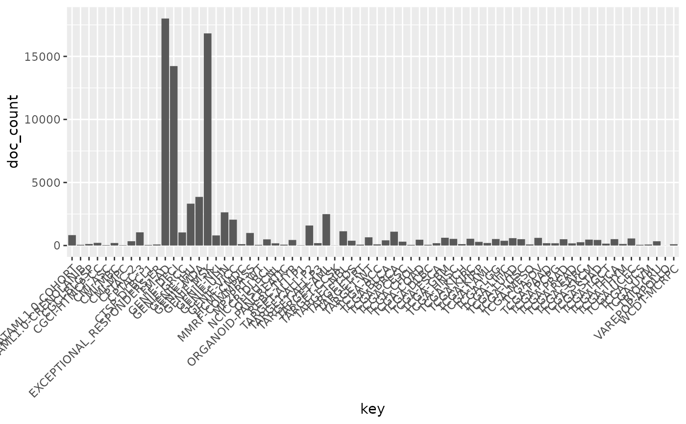
What is the breakdown of sample types in TCGA-BRCA?
# The need to do the "&" here is a requirement of the
# current version of the GDC API. I have filed a feature
# request to remove this requirement.
resp = cases() |> filter(~ project.project_id=='TCGA-BRCA' &
                              project.project_id=='TCGA-BRCA' ) |>
    facet('samples.sample_type') |> aggregations()
resp$samples.sample_type
## doc_count key
## 1 1098 primary tumor
## 2 1023 blood derived normal
## 3 162 solid tissue normal
## 4 7 metastaticFetch all samples in TCGA-BRCA that use “Solid Tissue” as a normal.
# The need to do the "&" here is a requirement of the
# current version of the GDC API. I have filed a feature
# request to remove this requirement.
resp = cases() |> filter(~ project.project_id=='TCGA-BRCA' &
                              samples.sample_type=='Solid Tissue Normal') |>
    GenomicDataCommons::select(c(default_fields(cases()),'samples.sample_type')) |>
    response_all()
count(resp)
## [1] 162## List of 1
## $ id: chr [1:162] "2021ed1f-dc75-4701-b8b8-1386466e4802" "20e8106b-1290-4735-abe4-7621e08e3dc8" "214a4507-d974-4b3e-8525-7408fccc6a0f" "21ef1730-e5a7-47ce-b419-d000bb59ae15" ...## [1] "2021ed1f-dc75-4701-b8b8-1386466e4802"
## [2] "20e8106b-1290-4735-abe4-7621e08e3dc8"
## [3] "214a4507-d974-4b3e-8525-7408fccc6a0f"
## [4] "21ef1730-e5a7-47ce-b419-d000bb59ae15"
## [5] "233b02f3-c4f0-4a67-9db5-e68d5cdaccb6"
## [6] "a2efe7e1-aca3-440f-825f-ed621edca69f"Get all TCGA case ids that are female
cases() |>
  GenomicDataCommons::filter(~ project.program.name == 'TCGA' &
    "cases.demographic.gender" %in% "female") |>
      GenomicDataCommons::results(size = 4) |>
        ids()
## [1] "4298ccdb-2e6d-4267-822d-75b021364084"
## [2] "439794a8-51bd-4c70-968c-34cf26b90148"
## [3] "305eaef4-4644-46e3-a696-d2e4a972f691"
## [4] "ec3b2a30-fcf6-45ef-bd9d-e6089a237c0f"Get all TCGA-COAD case ids that are NOT female
cases() |>
  GenomicDataCommons::filter(~ project.project_id == 'TCGA-COAD' &
    "cases.demographic.gender" %exclude% "female") |>
      GenomicDataCommons::results(size = 4) |>
        ids()
## [1] "265d7b06-65fe-42c5-ad21-e6b160e94718"
## [2] "d655bbf6-c710-411d-aff5-ceb0fb6e6680"
## [3] "4f601d7b-8db1-4c6d-9374-21dcd804980d"
## [4] "c085da47-d634-491a-80ea-514e5a231f70"Get all TCGA cases that are missing gender
cases() |>
  GenomicDataCommons::filter(~ project.program.name == 'TCGA' &
    missing("cases.demographic.gender")) |>
      GenomicDataCommons::results(size = 4) |>
        ids()
## [1] "a94de778-9c21-410d-8b9d-0f9240036bb8"
## [2] "f8360744-6bc8-4f53-b1fc-a133789455a8"
## [3] "1ec1e2c4-ba2c-40fc-b5e1-e8f6e38caec6"
## [4] "24506980-2857-4069-9af3-79ce4527eb00"Get all TCGA cases that are NOT missing gender
cases() |>
  GenomicDataCommons::filter(~ project.program.name == 'TCGA' &
    !missing("cases.demographic.gender")) |>
      GenomicDataCommons::results(size = 4) |>
        ids()
## [1] "4298ccdb-2e6d-4267-822d-75b021364084"
## [2] "a2663a86-a006-4867-9e88-2b523df48303"
## [3] "439794a8-51bd-4c70-968c-34cf26b90148"
## [4] "e865d40a-9989-436c-8426-88cc84c863e8"Files
How many of each type of file are available?
res = files() |> facet('type') |> aggregations()
res$type
## doc_count key
## 1 196351 annotated_somatic_mutation
## 2 174046 aligned_reads
## 3 136937 structural_variation
## 4 127458 simple_somatic_mutation
## 5 89858 copy_number_segment
## 6 51028 gene_expression
## 7 39593 aggregated_somatic_mutation
## 8 39002 copy_number_estimate
## 9 36556 mirna_expression
## 10 33476 slide_image
## 11 33146 masked_methylation_array
## 12 27344 biospecimen_supplement
## 13 24236 submitted_genotyping_array
## 14 23135 simple_germline_variation
## 15 21589 masked_somatic_mutation
## 16 16573 methylation_beta_value
## 17 16273 copy_number_auxiliary_file
## 18 14427 clinical_supplement
## 19 11324 pathology_report
## 20 7906 protein_expression
## 21 1426 submitted_expression_array
## 22 132 secondary_expression_analysis
ggplot(res$type,aes(x = key,y = doc_count)) + geom_bar(stat='identity') +
    theme(axis.text.x = element_text(angle = 45, hjust = 1))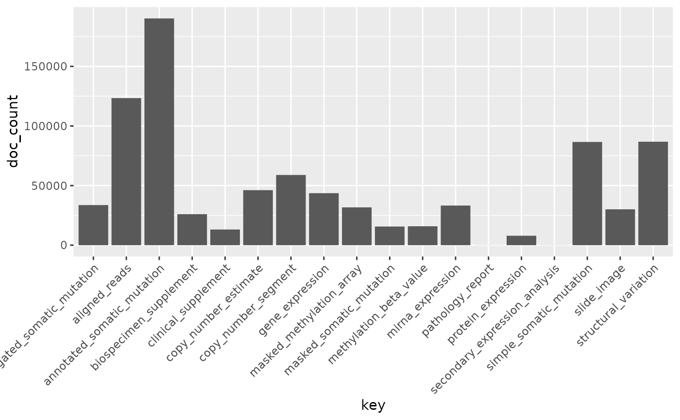
Find gene-level RNA-seq quantification files for GBM
q = files() |>
    GenomicDataCommons::select(available_fields('files')) |>
    filter(~ cases.project.project_id=='TCGA-GBM' &
               data_type=='Gene Expression Quantification')
q |> facet('analysis.workflow_type') |> aggregations()
## list()
# so need to add another filter
file_ids = q |> filter(~ cases.project.project_id=='TCGA-GBM' &
                            data_type=='Gene Expression Quantification' &
                            analysis.workflow_type == 'STAR - Counts') |>
    GenomicDataCommons::select('file_id') |>
    response_all() |>
    ids()
Slicing
Get all BAM file ids from TCGA-GBM
I need to figure out how to do slicing reproducibly in a testing environment and for vignette building.
q = files() |>
    GenomicDataCommons::select(available_fields('files')) |>
    filter(~ cases.project.project_id == 'TCGA-GBM' &
               data_type == 'Aligned Reads' &
               experimental_strategy == 'RNA-Seq' &
               data_format == 'BAM')
file_ids = q |> response_all() |> ids()
bamfile = slicing(file_ids[1],regions="chr12:6534405-6538375",token=gdc_token())
library(GenomicAlignments)
aligns = readGAlignments(bamfile)
Troubleshooting
SSL connection errors
- Symptom: Trying to connect to the API results in:
Error in curl::curl_fetch_memory(url, handle = handle) :
SSL connect error- Possible solutions: The issue is that the GDC
supports only recent security Transport Layer Security (TLS), so the
only known fix is to upgrade the system
opensslto version 1.0.1 or later.- [Mac OS],
- [Ubuntu]
-
[Centos/RHEL].
After upgrading
openssl, reinstall the Rcurlandhttrpackages.
sessionInfo()
## R version 4.4.2 (2024-10-31)
## Platform: x86_64-pc-linux-gnu
## Running under: Ubuntu 24.04.1 LTS
##
## Matrix products: default
## BLAS:   /usr/lib/x86_64-linux-gnu/openblas-pthread/libblas.so.3
## LAPACK: /usr/lib/x86_64-linux-gnu/openblas-pthread/libopenblasp-r0.3.26.so;  LAPACK version 3.12.0
##
## locale:
##  [1] LC_CTYPE=en_US.UTF-8       LC_NUMERIC=C
##  [3] LC_TIME=en_US.UTF-8        LC_COLLATE=en_US.UTF-8
##  [5] LC_MONETARY=en_US.UTF-8    LC_MESSAGES=en_US.UTF-8
##  [7] LC_PAPER=en_US.UTF-8       LC_NAME=C
##  [9] LC_ADDRESS=C               LC_TELEPHONE=C
## [11] LC_MEASUREMENT=en_US.UTF-8 LC_IDENTIFICATION=C
##
## time zone: Etc/UTC
## tzcode source: system (glibc)
##
## attached base packages:
## [1] stats     graphics  grDevices utils     datasets  methods   base
##
## other attached packages:
## [1] ggplot2_3.5.1             GenomicDataCommons_1.30.1
## [3] knitr_1.49                BiocStyle_2.34.0
##
## loaded via a namespace (and not attached):
##  [1] utf8_1.2.4              rappdirs_0.3.3          sass_0.4.9
##  [4] generics_0.1.3          tidyr_1.3.1             xml2_1.3.6
##  [7] hms_1.1.3               digest_0.6.37           magrittr_2.0.3
## [10] grid_4.4.2              evaluate_1.0.3          bookdown_0.42
## [13] fastmap_1.2.0           jsonlite_1.8.9          GenomeInfoDb_1.42.3
## [16] BiocManager_1.30.25     httr_1.4.7              purrr_1.0.4
## [19] scales_1.3.0            UCSC.utils_1.2.0        textshaping_1.0.0
## [22] jquerylib_0.1.4         cli_3.6.3               crayon_1.5.3
## [25] rlang_1.1.5             XVector_0.46.0          munsell_0.5.1
## [28] withr_3.0.2             cachem_1.1.0            yaml_2.3.10
## [31] tools_4.4.2             tzdb_0.4.0              dplyr_1.1.4
## [34] colorspace_2.1-1        GenomeInfoDbData_1.2.13 BiocGenerics_0.52.0
## [37] curl_6.2.0              vctrs_0.6.5             R6_2.5.1
## [40] stats4_4.4.2            lifecycle_1.0.4         zlibbioc_1.52.0
## [43] S4Vectors_0.44.0        fs_1.6.5                htmlwidgets_1.6.4
## [46] IRanges_2.40.1          ragg_1.3.3              pkgconfig_2.0.3
## [49] desc_1.4.3              gtable_0.3.6            pkgdown_2.1.1
## [52] bslib_0.9.0             pillar_1.10.1           glue_1.8.0
## [55] systemfonts_1.2.1       xfun_0.50               tibble_3.2.1
## [58] GenomicRanges_1.58.0    tidyselect_1.2.1        farver_2.1.2
## [61] htmltools_0.5.8.1       labeling_0.4.3          rmarkdown_2.29
## [64] readr_2.1.5             compiler_4.4.2
Developer notes
- The
S3object-oriented programming paradigm is used. - We have adopted a functional programming style with functions and methods that often take an “object” as the first argument. This style lends itself to pipeline-style programming.
- The GenomicDataCommons package uses the alternative request format (POST) to allow very large request bodies.