Setup and data exploration
As said, we will use the the wild-type data from the Tal1 chimera experiment:
- Sample 5: E8.5 injected cells (tomato positive), pool 3
- Sample 6: E8.5 host cells (tomato negative), pool 3
- Sample 7: E8.5 injected cells (tomato positive), pool 4
- Sample 8: E8.5 host cells (tomato negative), pool 4
- Sample 9: E8.5 injected cells (tomato positive), pool 5
- Sample 10: E8.5 host cells (tomato negative), pool 5
Note that this is a paired design in which for each biological replicate (pool 3, 4, and 5), we have both host and injected cells.
We start by loading the data and doing a quick exploratory analysis, essentially applying the normalization and visualization techniques that we have seen in the previous lectures to all samples.
library(MouseGastrulationData)
sce <- WTChimeraData(samples=5:10, type = "processed")
sce
## class: SingleCellExperiment
## dim: 29453 20935
## metadata(0):
## assays(1): counts
## rownames(29453): ENSMUSG00000051951 ENSMUSG00000089699 ...
## ENSMUSG00000095742 tomato-td
## rowData names(2): ENSEMBL SYMBOL
## colnames(20935): cell_9769 cell_9770 ... cell_30702 cell_30703
## colData names(11): cell barcode ... doub.density sizeFactor
## reducedDimNames(2): pca.corrected.E7.5 pca.corrected.E8.5
## mainExpName: NULL
## altExpNames(0):
colData(sce)## DataFrame with 20935 rows and 11 columns
## cell barcode sample stage tomato
## <character> <character> <integer> <character> <logical>
## cell_9769 cell_9769 AAACCTGAGACTGTAA 5 E8.5 TRUE
## cell_9770 cell_9770 AAACCTGAGATGCCTT 5 E8.5 TRUE
## cell_9771 cell_9771 AAACCTGAGCAGCCTC 5 E8.5 TRUE
## cell_9772 cell_9772 AAACCTGCATACTCTT 5 E8.5 TRUE
## cell_9773 cell_9773 AAACGGGTCAACACCA 5 E8.5 TRUE
## ... ... ... ... ... ...
## cell_30699 cell_30699 TTTGTCACAGCTCGCA 10 E8.5 FALSE
## cell_30700 cell_30700 TTTGTCAGTCTAGTCA 10 E8.5 FALSE
## cell_30701 cell_30701 TTTGTCATCATCGGAT 10 E8.5 FALSE
## cell_30702 cell_30702 TTTGTCATCATTATCC 10 E8.5 FALSE
## cell_30703 cell_30703 TTTGTCATCCCATTTA 10 E8.5 FALSE
## pool stage.mapped celltype.mapped closest.cell
## <integer> <character> <character> <character>
## cell_9769 3 E8.25 Mesenchyme cell_24159
## cell_9770 3 E8.5 Endothelium cell_96660
## cell_9771 3 E8.5 Allantois cell_134982
## cell_9772 3 E8.5 Erythroid3 cell_133892
## cell_9773 3 E8.25 Erythroid1 cell_76296
## ... ... ... ... ...
## cell_30699 5 E8.5 Erythroid3 cell_38810
## cell_30700 5 E8.5 Surface ectoderm cell_38588
## cell_30701 5 E8.25 Forebrain/Midbrain/H.. cell_66082
## cell_30702 5 E8.5 Erythroid3 cell_138114
## cell_30703 5 E8.0 Doublet cell_92644
## doub.density sizeFactor
## <numeric> <numeric>
## cell_9769 0.02985045 1.41243
## cell_9770 0.00172753 1.22757
## cell_9771 0.01338013 1.15439
## cell_9772 0.00218402 1.28676
## cell_9773 0.00211723 1.78719
## ... ... ...
## cell_30699 0.00146287 0.389311
## cell_30700 0.00374155 0.588784
## cell_30701 0.05651258 0.624455
## cell_30702 0.00108837 0.550807
## cell_30703 0.82369305 1.184919To speed up computations, after removing doublets, we randomly select 50% cells per sample.
library(scater)
library(ggplot2)
library(scran)

# remove doublets
drop <- sce$celltype.mapped %in% c("stripped", "Doublet")
sce <- sce[,!drop]

set.seed(29482)
idx <- unlist(tapply(colnames(sce), sce$sample, function(x) {
    perc <- round(0.50 * length(x))
    sample(x, perc)
}))

sce <- sce[,idx]
We now normalize the data and visualize them in a tSNE plot.
# normalization
sce <- logNormCounts(sce)

# identify highly variable genes
dec <- modelGeneVar(sce, block=sce$sample)
chosen.hvgs <- dec$bio > 0

# dimensionality reduction
sce <- runPCA(sce, subset_row = chosen.hvgs, ntop = 1000)
sce <- runTSNE(sce, dimred = "PCA")

sce$sample <- as.factor(sce$sample)
plotTSNE(sce, colour_by = "sample")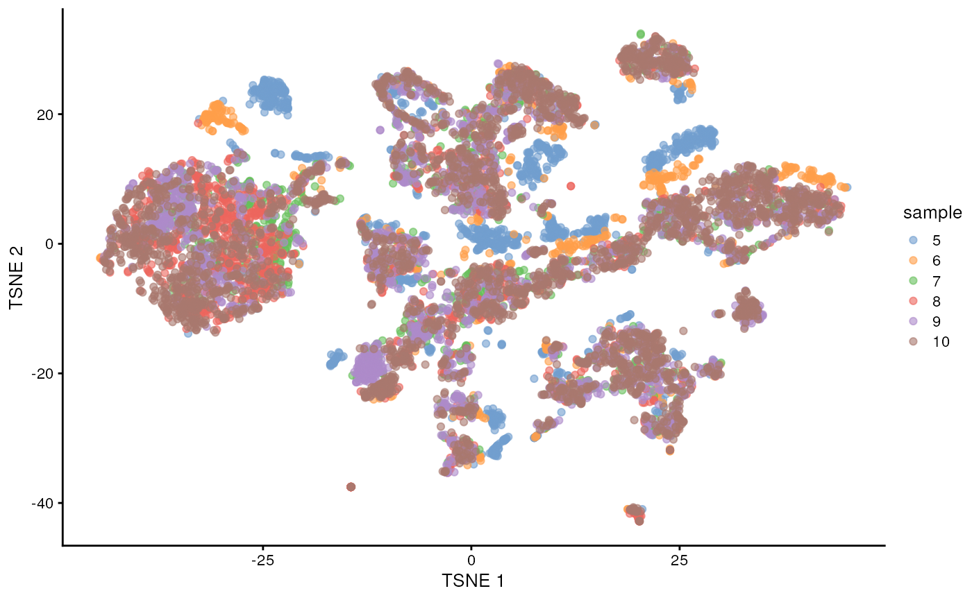
plotTSNE(sce, colour_by = "celltype.mapped") +
    scale_color_discrete() +
    theme(legend.position = "bottom")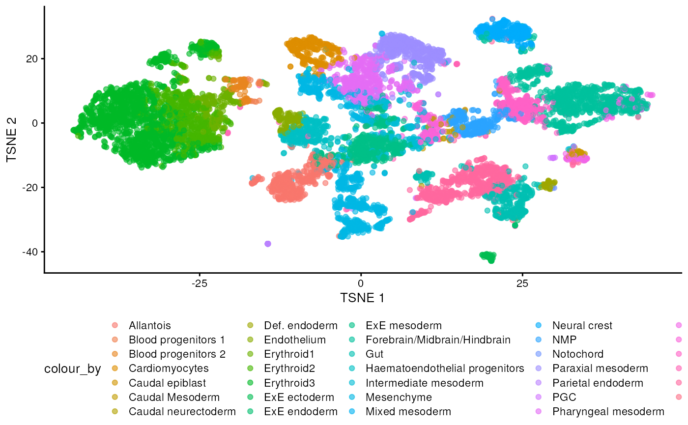
There are evident sample effects. Depending on the analysis that you want to perform you may want to remove or retain the sample effect. For instance, if the goal is to identify cell types with a clustering method, one may want to remove the sample effects with “batch effect” correction methods.
For now, let’s assume that we want to remove this effect.
Correcting batch effects
We correct the effect of samples by aid of the
correctExperiment function in the batchelor
package and using the sample colData column as
batch.
library(batchelor)
set.seed(10102)
merged <- correctExperiments(sce,
    batch=sce$sample,
    subset.row=chosen.hvgs,
    PARAM=FastMnnParam(
        merge.order=list(
            list(1,3,5), # WT (3 replicates)
            list(2,4,6)  # td-Tomato (3 replicates)
        )
    )
)

merged <- runTSNE(merged, dimred="corrected")
plotTSNE(merged, colour_by="batch")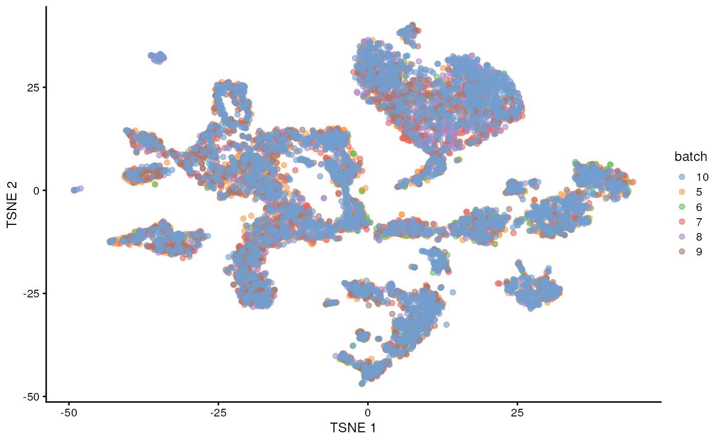
Once we removed the sample batch effect, we can proceed with the Differential Expression Analysis.
Differential Expression
In order to perform a Differential Expression Analysis, we need to identify groups of cells across samples/conditions (depending on the experimental design and the final aim of the experiment).
As previously seen, we have two ways of grouping cells, cell clustering and cell labeling. In our case we will focus on this second aspect to group cells according to the already annotated cell types to proceed with the computation of the pseudo-bulk samples.
Pseudo-bulk samples
To compute differences between groups of cells, a possible way is to compute pseudo-bulk samples, where we mediate the gene signal of all the cells for each specific cell type. In this manner, we are then able to detect differences between the same cell type across two different conditions.
To compute pseudo-bulk samples, we use the
aggregateAcrossCells function in the scuttle
package, which takes as input not only a SingleCellExperiment, but also
the id to use for the identification of the group of cells. In our case,
we use as id not just the cell type, but also the sample, because we
want be able to discern between replicates and conditions during further
steps.
# Using 'label' and 'sample' as our two factors; each column of the output
# corresponds to one unique combination of these two factors.
library(scuttle)
summed <- aggregateAcrossCells(merged,
    id=colData(merged)[,c("celltype.mapped", "sample")])
summed
## class: SingleCellExperiment
## dim: 13641 179
## metadata(2): merge.info pca.info
## assays(1): counts
## rownames(13641): ENSMUSG00000051951 ENSMUSG00000025900 ...
## ENSMUSG00000096730 ENSMUSG00000095742
## rowData names(3): rotation ENSEMBL SYMBOL
## colnames: NULL
## colData names(15): batch cell ... sample ncells
## reducedDimNames(5): corrected pca.corrected.E7.5 pca.corrected.E8.5 PCA
## TSNE
## mainExpName: NULL
## altExpNames(0):Differential Expression Analysis
The main advantage of using pseudo-bulk samples is the possibility to
use well-tested methods for differential analysis like
edgeR and DESeq2, we will focus on the former
for this analysis. edgeR uses a Negative Binomial
Generalized Linear Model.
First, let’s start with a specific cell type, for instance the “Mesenchymal stem cells”, and look into differences between this cell type across conditions.
label <- "Mesenchyme"
current <- summed[,label==summed$celltype.mapped]

# Creating up a DGEList object for use in edgeR:
library(edgeR)
y <- DGEList(counts(current), samples=colData(current))
y
## An object of class "DGEList"
## $counts
## Sample1 Sample2 Sample3 Sample4 Sample5 Sample6
## ENSMUSG00000051951 2 0 0 0 1 0
## ENSMUSG00000025900 0 0 0 0 0 0
## ENSMUSG00000025902 4 0 2 0 3 6
## ENSMUSG00000033845 765 130 508 213 781 305
## ENSMUSG00000002459 2 0 1 0 0 0
## 13636 more rows ...
##
## $samples
## group lib.size norm.factors batch cell barcode sample stage tomato pool
## Sample1 1 2478901 1 5 <NA> <NA> 5 E8.5 TRUE 3
## Sample2 1 548407 1 6 <NA> <NA> 6 E8.5 FALSE 3
## Sample3 1 1260187 1 7 <NA> <NA> 7 E8.5 TRUE 4
## Sample4 1 578699 1 8 <NA> <NA> 8 E8.5 FALSE 4
## Sample5 1 2092329 1 9 <NA> <NA> 9 E8.5 TRUE 5
## Sample6 1 904929 1 10 <NA> <NA> 10 E8.5 FALSE 5
## stage.mapped celltype.mapped closest.cell doub.density sizeFactor
## Sample1 <NA> Mesenchyme <NA> NA NA
## Sample2 <NA> Mesenchyme <NA> NA NA
## Sample3 <NA> Mesenchyme <NA> NA NA
## Sample4 <NA> Mesenchyme <NA> NA NA
## Sample5 <NA> Mesenchyme <NA> NA NA
## Sample6 <NA> Mesenchyme <NA> NA NA
## celltype.mapped.1 sample.1 ncells
## Sample1 Mesenchyme 5 151
## Sample2 Mesenchyme 6 28
## Sample3 Mesenchyme 7 127
## Sample4 Mesenchyme 8 75
## Sample5 Mesenchyme 9 239
## Sample6 Mesenchyme 10 146A typical step is to discard low quality samples due to low sequenced library size. We discard these samples because they can affect further steps like normalization and/or DEGs analysis.
We can see that in our case we don’t have low quality samples and we don’t need to filter out any of them.
discarded <- current$ncells < 10
y <- y[,!discarded]
summary(discarded)
## Mode FALSE
## logical 6The same idea is typically applied to the genes, indeed we need to discard low expressed genes to improve accuracy for the DEGs modeling.
keep <- filterByExpr(y, group=current$tomato)
y <- y[keep,]
summary(keep)
## Mode FALSE TRUE
## logical 9121 4520We can now proceed to normalize the data There are several approaches
for normalizing bulk, and hence pseudo-bulk data. Here, we use the
Trimmed Mean of M-values method, implemented in the edgeR
package within the calcNormFactors function. Keep in mind
that because we are going to normalize the pseudo-bulk counts, we don’t
need to normalize the data in “single cell form”.
y <- calcNormFactors(y)
y$samples
## group lib.size norm.factors batch cell barcode sample stage tomato pool
## Sample1 1 2478901 1.0506857 5 <NA> <NA> 5 E8.5 TRUE 3
## Sample2 1 548407 1.0399112 6 <NA> <NA> 6 E8.5 FALSE 3
## Sample3 1 1260187 0.9700083 7 <NA> <NA> 7 E8.5 TRUE 4
## Sample4 1 578699 0.9871129 8 <NA> <NA> 8 E8.5 FALSE 4
## Sample5 1 2092329 0.9695559 9 <NA> <NA> 9 E8.5 TRUE 5
## Sample6 1 904929 0.9858611 10 <NA> <NA> 10 E8.5 FALSE 5
## stage.mapped celltype.mapped closest.cell doub.density sizeFactor
## Sample1 <NA> Mesenchyme <NA> NA NA
## Sample2 <NA> Mesenchyme <NA> NA NA
## Sample3 <NA> Mesenchyme <NA> NA NA
## Sample4 <NA> Mesenchyme <NA> NA NA
## Sample5 <NA> Mesenchyme <NA> NA NA
## Sample6 <NA> Mesenchyme <NA> NA NA
## celltype.mapped.1 sample.1 ncells
## Sample1 Mesenchyme 5 151
## Sample2 Mesenchyme 6 28
## Sample3 Mesenchyme 7 127
## Sample4 Mesenchyme 8 75
## Sample5 Mesenchyme 9 239
## Sample6 Mesenchyme 10 146To investigate the effect of our normalization, we use a Mean-Difference (MD) plot for each sample in order to detect possible normalization problems due to insufficient cells/reads/UMIs composing a particular pseudo-bulk profile.
In our case, we verify that all these plots are centered in 0 (on y-axis) and present a trumpet shape, as expected.

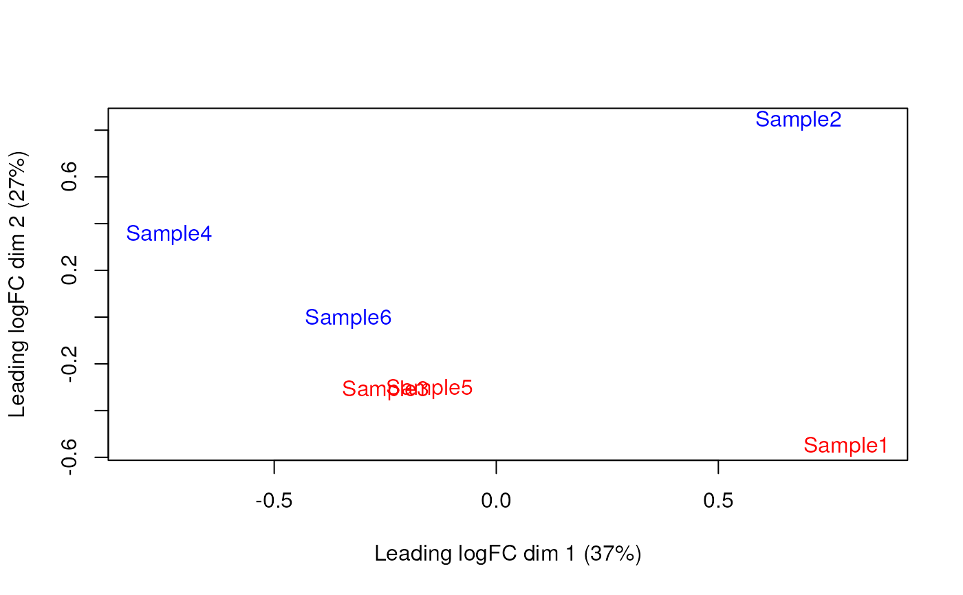
Furthermore, we want to check if the samples cluster together based on their known factors (like the tomato injection in this case).
To do so, we use the MDS plot, which is very close to a PCA representation.
We then construct a design matrix by including both the pool and the tomato as factors. This design indicates which samples belong to which pool and condition, so we can use it in the next step of the analysis.
design <- model.matrix(~factor(pool) + factor(tomato), y$samples)
design
## (Intercept) factor(pool)4 factor(pool)5 factor(tomato)TRUE
## Sample1 1 0 0 1
## Sample2 1 0 0 0
## Sample3 1 1 0 1
## Sample4 1 1 0 0
## Sample5 1 0 1 1
## Sample6 1 0 1 0
## attr(,"assign")
## [1] 0 1 1 2
## attr(,"contrasts")
## attr(,"contrasts")$`factor(pool)`
## [1] "contr.treatment"
##
## attr(,"contrasts")$`factor(tomato)`
## [1] "contr.treatment"Now we can estimate the Negative Binomial (NB) overdispersion parameter, to model the mean-variance trend.
y <- estimateDisp(y, design)
summary(y$trended.dispersion)
## Min. 1st Qu. Median Mean 3rd Qu. Max.
## 0.009325 0.016271 0.024233 0.021603 0.026868 0.027993The BCV plot allows us to investigate the relation between the
Biological Coefficient of Variation and the Average log CPM for each
gene. Additionally, the Common and Trend BCV are shown in
red and blue.
plotBCV(y)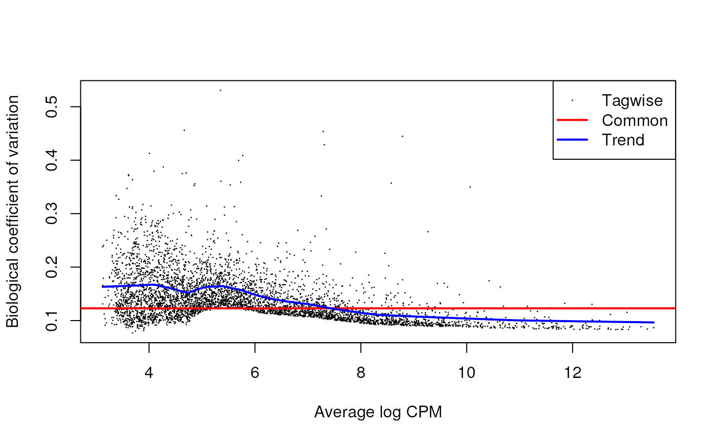
We then fit a Quasi-Likelihood (QL) negative binomial generalized
linear model for each gene. The robust=TRUE parameter
avoids distorsions from highly variable clusters. The QL method includes
an additional dispersion parameter, useful to handle the uncertainty and
variability of the per-gene variance, which is not well estimated by the
NB dispersions, so the two dispersion types complement each other in the
final analysis.
##    Min. 1st Qu.  Median    Mean 3rd Qu.    Max.
##  0.2977  0.6640  0.8275  0.7637  0.8798  0.9670
summary(fit$df.prior)## Min. 1st Qu. Median Mean 3rd Qu. Max.
## 0.323 8.177 8.177 8.111 8.177 8.177QL dispersion estimates for each gene as a function of abundance. Raw estimates (black) are shrunk towards the trend (blue) to yield squeezed estimates (red).
plotQLDisp(fit)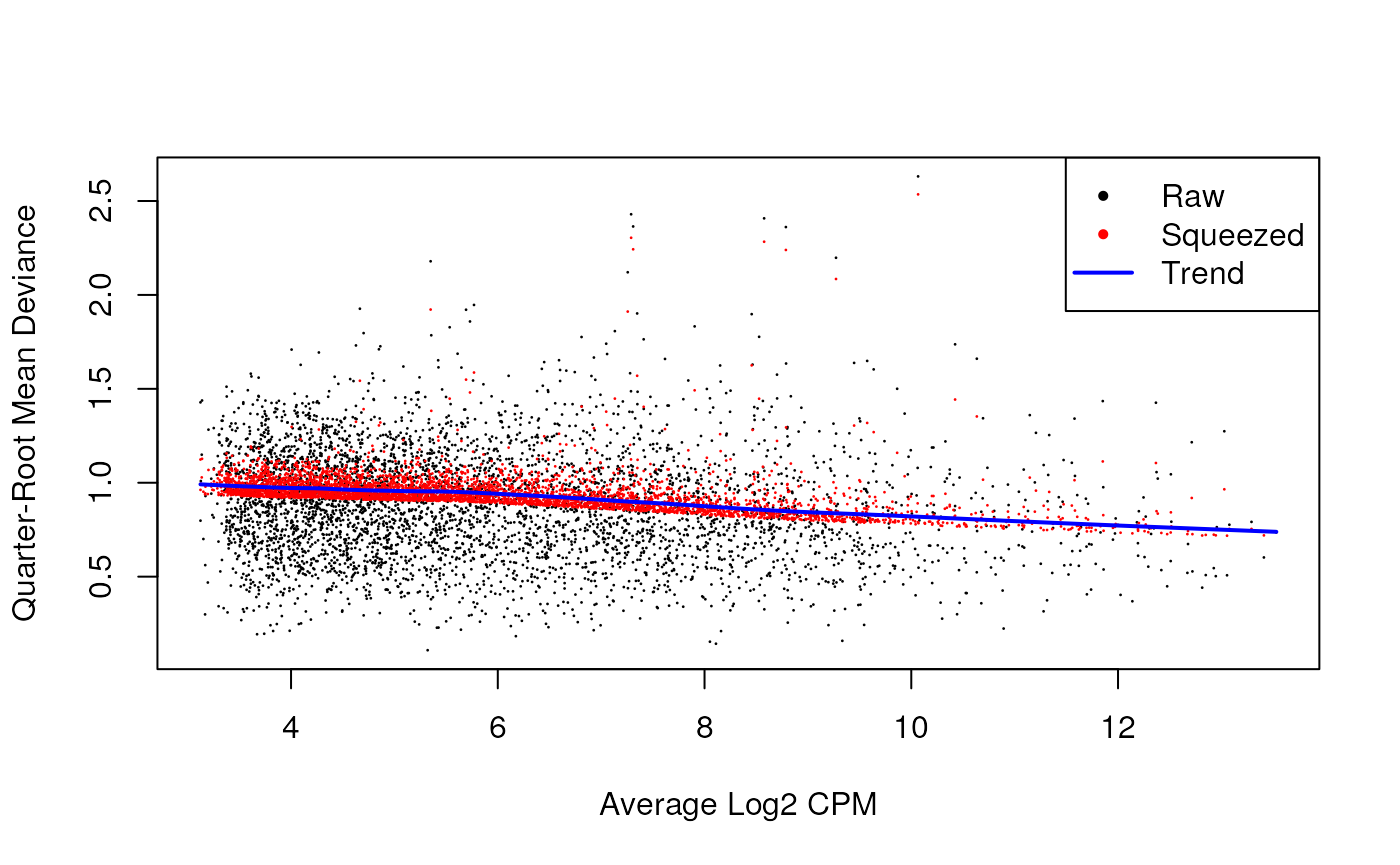
We then use an empirical Bayes quasi-likelihood F-test to test for differential expression (due to tomato injection) per each gene at a False Discovery Rate (FDR) of 5%. The low amount of DGEs highlights that the tomato injection effect has a low influence on the mesenchyme cells.
res <- glmQLFTest(fit, coef=ncol(design))
summary(decideTests(res))
## factor(tomato)TRUE
## Down 5
## NotSig 4510
## Up 5
topTags(res)## Coefficient: factor(tomato)TRUE
## logFC logCPM F PValue FDR
## ENSMUSG00000010760 -4.1551264 9.973704 1112.14948 9.905998e-12 4.477511e-08
## ENSMUSG00000096768 1.9992920 8.844258 403.85294 1.594095e-09 3.602655e-06
## ENSMUSG00000035299 1.8001627 6.904163 123.52980 5.130084e-07 7.729327e-04
## ENSMUSG00000101609 1.3708397 7.310009 80.58075 3.745290e-06 4.232177e-03
## ENSMUSG00000019188 -1.0195649 7.545530 61.65538 1.248303e-05 1.128466e-02
## ENSMUSG00000024423 0.9946833 7.391075 58.34967 1.591674e-05 1.199061e-02
## ENSMUSG00000086503 -6.5155131 7.411257 159.33690 2.625600e-05 1.695388e-02
## ENSMUSG00000042607 -0.9567347 7.468203 45.42154 4.690293e-05 2.650016e-02
## ENSMUSG00000036446 -0.8305889 9.401028 42.72058 6.071290e-05 3.049137e-02
## ENSMUSG00000027520 1.5814592 6.952923 40.94715 7.775888e-05 3.514702e-02All the previous steps can be easily performed with the following
function for each cell type, thanks to the pseudoBulkDGE
function in the scran package.
library(scran)
summed.filt <- summed[,summed$ncells >= 10]

de.results <- pseudoBulkDGE(summed.filt,
    label=summed.filt$celltype.mapped,
    design=~factor(pool) + tomato,
    coef="tomatoTRUE",
    condition=summed.filt$tomato
)
The returned object is a list of DataFrames each with
the results for a cell type. Each of these contains also the
intermediate results in edgeR format to perform any
intermediate plot or diagnostic.
cur.results <- de.results[["Allantois"]]
cur.results[order(cur.results$PValue),]
## DataFrame with 13641 rows and 5 columns
## logFC logCPM F PValue FDR
## <numeric> <numeric> <numeric> <numeric> <numeric>
## ENSMUSG00000037664 -7.995130 11.55290 3180.990 7.35933e-22 3.09165e-18
## ENSMUSG00000010760 -2.574762 12.40592 1114.529 9.22901e-18 1.93855e-14
## ENSMUSG00000086503 -7.015319 7.49749 703.373 5.57372e-16 7.80507e-13
## ENSMUSG00000096768 1.828480 9.33239 304.769 8.39747e-13 8.81944e-10
## ENSMUSG00000022464 0.969837 10.28302 118.697 2.12502e-09 1.78544e-06
## ... ... ... ... ... ...
## ENSMUSG00000095247 NA NA NA NA NA
## ENSMUSG00000096808 NA NA NA NA NA
## ENSMUSG00000079808 NA NA NA NA NA
## ENSMUSG00000096730 NA NA NA NA NA
## ENSMUSG00000095742 NA NA NA NA NADifferential Abundance
With DA we test for differences between clusters across conditions, to investigate which clusters change accordingly to the treatment (the tomato injection in our case).
We first setup some code and variables for further analysis, like quantifying the number of cells per each cell type and fit a model to catch differences between the injected cells and the background.
The performed steps are very similar to the ones for DEGs analysis, but this time we start our analysis on the computed abundances and without normalizing the data with TMM.
library(edgeR)
abundances <- table(merged$celltype.mapped, merged$sample)
abundances <- unclass(abundances)
# Attaching some column metadata.
extra.info <- colData(merged)[match(colnames(abundances), merged$sample),]
y.ab <- DGEList(abundances, samples=extra.info)

design <- model.matrix(~factor(pool) + factor(tomato), y.ab$samples)
y.ab <- estimateDisp(y.ab, design, trend="none")
fit.ab <- glmQLFit(y.ab, design, robust=TRUE, abundance.trend=FALSE)
Background on compositional effect
As mentioned before, in DA we don’t normalize our data with
calcNormFactors function, because this approach considers
that most of the input features do not vary between conditions. This
cannot be applied to this analysis because we have a small number of
cell populations that all can change due to the treatment. Leaving us to
normalize only for library depth, which in pseudo-bulk data means by the
total number of cells in each sample (cell type).
On the other hand, this can lead our data to be susceptible to compositional effect, that means that our conclusions can be biased by the amount of cells present in each cell type. And this amount of cells can be totally unbalanced between cell types.
For example, a specific cell type can be 40% of the total amount of cells present in the experiment, while another just the 3%. The differences in terms of abundance of these cell types are detected between the different conditions, but our final interpretation could be biased if we don’t consider this aspect.
We now look at different approaches for handling the compositional effect.
Assuming most labels do not change
We can use a similar approach used during the DEGs analysis, assuming that most labels are not changing, in particular if we think about the low number of DEGs resulted from the previous analysis.
To do so, we first normalize the data with
calcNormFactors and then we fit and estimate a QL-model for
our abundance data.
y.ab2 <- calcNormFactors(y.ab)
y.ab2$samples$norm.factors
## [1] 1.1029040 1.0228173 1.0695358 0.7686501 1.0402941 1.0365354We then follow the already seen edgeR analysis steps.
y.ab2 <- estimateDisp(y.ab2, design, trend="none")
fit.ab2 <- glmQLFit(y.ab2, design, robust=TRUE, abundance.trend=FALSE)
res2 <- glmQLFTest(fit.ab2, coef=ncol(design))
summary(decideTests(res2))
## factor(tomato)TRUE
## Down 2
## NotSig 32
## Up 0
topTags(res2, n=10)## Coefficient: factor(tomato)TRUE
## logFC logCPM F PValue FDR
## ExE ectoderm -5.7452733 13.13490 37.367234 5.393309e-08 1.833725e-06
## Parietal endoderm -6.9016375 12.36649 25.884039 3.062123e-06 5.205609e-05
## Mesenchyme 0.9656118 16.32654 6.139328 1.570983e-02 1.495573e-01
## Erythroid3 -0.9192068 17.34677 5.921070 1.759497e-02 1.495573e-01
## Neural crest -1.0200609 14.83912 5.276218 2.470370e-02 1.679851e-01
## ExE endoderm -3.9992127 10.75172 4.673383 3.415631e-02 1.935524e-01
## Endothelium 0.8666732 14.12195 3.307087 7.338557e-02 3.564442e-01
## Cardiomyocytes 0.6956771 14.93321 2.592279 1.120186e-01 4.760789e-01
## Allantois 0.6001360 15.54924 2.085500 1.532954e-01 5.791158e-01
## Erythroid2 -0.5177901 15.97357 1.614924 2.081314e-01 7.076469e-01Testing against a log-fold change threshold
This other approach assumes that the composition bias introduces a spurious log2-fold change of no more than a quantity for a non-DA label. In other words, we interpret this as the maximum log-fold change in the total number of cells given by DA in other labels. On the other hand, when choosing , we should not consider fold-differences in the totals due to differences in capture efficiency or the size of the original cell population are not attributable to composition bias. We then mitigate the effect of composition biases by testing each label for changes in abundance beyond .
res.lfc <- glmTreat(fit.ab, coef=ncol(design), lfc=1)
summary(decideTests(res.lfc))
## factor(tomato)TRUE
## Down 2
## NotSig 32
## Up 0
topTags(res.lfc)## Coefficient: factor(tomato)TRUE
## logFC unshrunk.logFC logCPM PValue
## ExE ectoderm -5.4835385 -5.9123463 13.06465 4.691927e-06
## Parietal endoderm -6.5773855 -27.4596643 12.30091 8.041229e-05
## ExE endoderm -3.9301490 -23.9290916 10.76159 5.050518e-02
## Mesenchyme 1.1597987 1.1610214 16.35239 1.509665e-01
## Endothelium 1.0396400 1.0450849 14.14422 2.268038e-01
## Caudal neurectoderm -1.4805723 -1.6367540 11.09613 2.934582e-01
## Cardiomyocytes 0.8713101 0.8740177 14.96579 3.377083e-01
## Neural crest -0.8238482 -0.8264411 14.83184 3.713878e-01
## Allantois 0.8033893 0.8048744 15.54528 3.952001e-01
## Def. endoderm 0.7098640 0.7228811 12.50001 4.365468e-01
## FDR
## ExE ectoderm 0.0001595255
## Parietal endoderm 0.0013670090
## ExE endoderm 0.5723920586
## Mesenchyme 0.9906682053
## Endothelium 0.9906682053
## Caudal neurectoderm 0.9906682053
## Cardiomyocytes 0.9906682053
## Neural crest 0.9906682053
## Allantois 0.9906682053
## Def. endoderm 0.9906682053Addionally, the choice of can be guided by other external experimental data, like a previous or a pilot experiment.
Session Info
## R version 4.3.0 (2023-04-21)
## Platform: x86_64-pc-linux-gnu (64-bit)
## Running under: Ubuntu 22.04.2 LTS
##
## Matrix products: default
## BLAS:   /usr/lib/x86_64-linux-gnu/openblas-pthread/libblas.so.3
## LAPACK: /usr/lib/x86_64-linux-gnu/openblas-pthread/libopenblasp-r0.3.20.so;  LAPACK version 3.10.0
##
## locale:
##  [1] LC_CTYPE=en_US.UTF-8       LC_NUMERIC=C
##  [3] LC_TIME=en_US.UTF-8        LC_COLLATE=en_US.UTF-8
##  [5] LC_MONETARY=en_US.UTF-8    LC_MESSAGES=en_US.UTF-8
##  [7] LC_PAPER=en_US.UTF-8       LC_NAME=C
##  [9] LC_ADDRESS=C               LC_TELEPHONE=C
## [11] LC_MEASUREMENT=en_US.UTF-8 LC_IDENTIFICATION=C
##
## time zone: Etc/UTC
## tzcode source: system (glibc)
##
## attached base packages:
## [1] stats4    stats     graphics  grDevices utils     datasets  methods
## [8] base
##
## other attached packages:
##  [1] edgeR_3.42.4                 limma_3.56.2
##  [3] batchelor_1.16.0             scran_1.28.1
##  [5] scater_1.28.0                ggplot2_3.4.2
##  [7] scuttle_1.10.1               MouseGastrulationData_1.14.0
##  [9] SpatialExperiment_1.10.0     SingleCellExperiment_1.22.0
## [11] SummarizedExperiment_1.30.2  Biobase_2.60.0
## [13] GenomicRanges_1.52.0         GenomeInfoDb_1.36.1
## [15] IRanges_2.34.1               S4Vectors_0.38.1
## [17] BiocGenerics_0.46.0          MatrixGenerics_1.12.2
## [19] matrixStats_1.0.0            BiocStyle_2.28.0
##
## loaded via a namespace (and not attached):
##   [1] jsonlite_1.8.7                magrittr_2.0.3
##   [3] ggbeeswarm_0.7.2              magick_2.7.4
##   [5] farver_2.1.1                  rmarkdown_2.23
##   [7] fs_1.6.2                      zlibbioc_1.46.0
##   [9] ragg_1.2.5                    vctrs_0.6.3
##  [11] memoise_2.0.1                 DelayedMatrixStats_1.22.1
##  [13] RCurl_1.98-1.12               htmltools_0.5.5
##  [15] S4Arrays_1.0.4                AnnotationHub_3.8.0
##  [17] curl_5.0.1                    BiocNeighbors_1.18.0
##  [19] Rhdf5lib_1.22.0               rhdf5_2.44.0
##  [21] sass_0.4.6                    bslib_0.5.0
##  [23] desc_1.4.2                    cachem_1.0.8
##  [25] ResidualMatrix_1.10.0         igraph_1.5.0
##  [27] mime_0.12                     lifecycle_1.0.3
##  [29] pkgconfig_2.0.3               rsvd_1.0.5
##  [31] Matrix_1.6-0                  R6_2.5.1
##  [33] fastmap_1.1.1                 GenomeInfoDbData_1.2.10
##  [35] shiny_1.7.4.1                 digest_0.6.33
##  [37] colorspace_2.1-0              AnnotationDbi_1.62.2
##  [39] rprojroot_2.0.3               dqrng_0.3.0
##  [41] irlba_2.3.5.1                 ExperimentHub_2.8.0
##  [43] textshaping_0.3.6             RSQLite_2.3.1
##  [45] beachmat_2.16.0               labeling_0.4.2
##  [47] filelock_1.0.2                fansi_1.0.4
##  [49] httr_1.4.6                    compiler_4.3.0
##  [51] bit64_4.0.5                   withr_2.5.0
##  [53] BiocParallel_1.34.2           viridis_0.6.3
##  [55] DBI_1.1.3                     highr_0.10
##  [57] HDF5Array_1.28.1              R.utils_2.12.2
##  [59] rappdirs_0.3.3                DelayedArray_0.26.6
##  [61] bluster_1.10.0                rjson_0.2.21
##  [63] tools_4.3.0                   vipor_0.4.5
##  [65] beeswarm_0.4.0                interactiveDisplayBase_1.38.0
##  [67] httpuv_1.6.11                 R.oo_1.25.0
##  [69] glue_1.6.2                    rhdf5filters_1.12.1
##  [71] promises_1.2.0.1              grid_4.3.0
##  [73] Rtsne_0.16                    cluster_2.1.4
##  [75] generics_0.1.3                gtable_0.3.3
##  [77] R.methodsS3_1.8.2             metapod_1.8.0
##  [79] BiocSingular_1.16.0           ScaledMatrix_1.8.1
##  [81] utf8_1.2.3                    XVector_0.40.0
##  [83] ggrepel_0.9.3                 BiocVersion_3.17.1
##  [85] pillar_1.9.0                  stringr_1.5.0
##  [87] BumpyMatrix_1.8.0             later_1.3.1
##  [89] splines_4.3.0                 dplyr_1.1.2
##  [91] BiocFileCache_2.8.0           lattice_0.21-8
##  [93] bit_4.0.5                     tidyselect_1.2.0
##  [95] locfit_1.5-9.8                Biostrings_2.68.1
##  [97] knitr_1.43                    gridExtra_2.3
##  [99] xfun_0.39                     statmod_1.5.0
## [101] DropletUtils_1.20.0           stringi_1.7.12
## [103] yaml_2.3.7                    evaluate_0.21
## [105] codetools_0.2-19              tibble_3.2.1
## [107] BiocManager_1.30.21           cli_3.6.1
## [109] xtable_1.8-4                  systemfonts_1.0.4
## [111] munsell_0.5.0                 jquerylib_0.1.4
## [113] Rcpp_1.0.11                   dbplyr_2.3.3
## [115] png_0.1-8                     parallel_4.3.0
## [117] ellipsis_0.3.2                pkgdown_2.0.7
## [119] blob_1.2.4                    sparseMatrixStats_1.12.2
## [121] bitops_1.0-7                  viridisLite_0.4.2
## [123] scales_1.2.1                  purrr_1.0.1
## [125] crayon_1.5.2                  rlang_1.1.1
## [127] formatR_1.14                  cowplot_1.1.1
## [129] KEGGREST_1.40.0
Further Reading
- OSCA book, Multi-sample analysis, Chapters 1, 4, and 6