Accessing data from the Human Cell Atlas (HCA)

HCA Project

The Human Cell Atlas (HCA) is a large project that aims to learn from and map every cell type in the human body. The project extracts spatial and molecular characteristics in order to understand cellular function and networks. It is an international collaborative that charts healthy cells in the human body at all ages. There are about 37.2 trillion cells in the human body. To read more about the project, head over to their website at https://www.humancellatlas.org.

CELLxGENE

CELLxGENE is a database and a suite of tools that help scientists to find, download, explore, analyze, annotate, and publish single cell data. It includes several analytic and visualization tools to help you to discover single cell data patterns. To see the list of tools, browse to https://cellxgene.cziscience.com/.

CELLxGENE | Census

The Census provides efficient computational tooling to access, query, and analyze all single-cell RNA data from CZ CELLxGENE Discover. Using a new access paradigm of cell-based slicing and querying, you can interact with the data through TileDB-SOMA, or get slices in AnnData or Seurat objects, thus accelerating your research by significantly minimizing data harmonization at https://chanzuckerberg.github.io/cellxgene-census/.

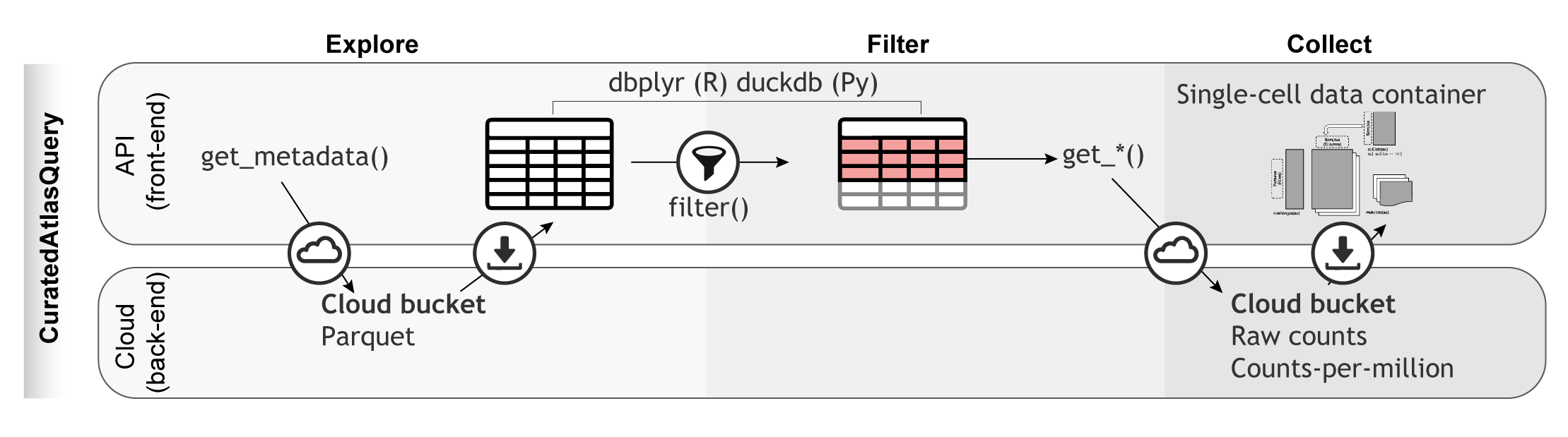
The CuratedAtlasQueryR Project

To systematically characterize the immune system across tissues, demographics and multiple studies, single cell transcriptomics data was harmonized from the CELLxGENE database. Data from 28,975,366 cells that cover 156 tissues (excluding cell cultures), 12,981 samples, and 324 studies were collected. The metadata was standardized, including sample identifiers, tissue labels (based on anatomy) and age. Also, the gene-transcript abundance of all samples was harmonized by putting values on the positive natural scale (i.e. non-logarithmic).

To model the immune system across studies, we adopted a consistent immune cell-type ontology appropriate for lymphoid and non-lymphoid tissues. We applied a consensus cell labeling strategy between the Seurat blueprint and Monaco (2019) to minimize biases in immune cell classification from study-specific standards.

CuratedAtlasQueryR supports data access and programmatic exploration of the harmonized atlas. Cells of interest can be selected based on ontology, tissue of origin, demographics, and disease. For example, the user can select CD4 T helper cells across healthy and diseased lymphoid tissue. The data for the selected cells can be downloaded locally into popular single-cell data containers. Pseudo bulk counts are also available to facilitate large-scale, summary analyses of transcriptional profiles. This platform offers a standardized workflow for accessing atlas-level datasets programmatically and reproducibly.

Data Sources in R / Bioconductor

There are a few options to access single cell data with R / Bioconductor.

Package	Target	Description
hca	HCA Data Portal API	Project, Sample, and File level HCA data
cellxgenedp	CellxGene	Human and mouse SC data including HCA
CuratedAtlasQueryR	CellxGene	fine-grained query capable CELLxGENE data including HCA

Installation

if (!requireNamespace("BiocManager", quietly = TRUE))
    install.packages("BiocManager")

BiocManager::install("stemangiola/CuratedAtlasQueryR")

Package load

library(CuratedAtlasQueryR)
library(dplyr)

HCA Metadata

The metadata allows the user to get a lay of the land of what is available via the package. In this example, we are using the sample database URL which allows us to get a small and quick subset of the available metadata.

metadata <- get_metadata(remote_url = CuratedAtlasQueryR::SAMPLE_DATABASE_URL)

Get a view of the first 10 columns in the metadata with glimpse

metadata |>
  select(1:10) |>
  glimpse()

## Rows: ??
## Columns: 10
## Database: DuckDB 0.8.1 [unknown@Linux 5.15.0-1041-azure:R 4.3.0/:memory:]
## $ cell_                             <chr> "TTATGCTAGGGTGTTG_12", "GCTTGAACATGG…
## $ sample_                           <chr> "039c558ca1c43dc74c563b58fe0d6289", …
## $ cell_type                         <chr> "mature NK T cell", "mature NK T cel…
## $ cell_type_harmonised              <chr> "immune_unclassified", "cd8 tem", "i…
## $ confidence_class                  <dbl> 5, 3, 5, 5, 5, 5, 5, 5, 5, 5, 5, 1, …
## $ cell_annotation_azimuth_l2        <chr> "gdt", "cd8 tem", "cd8 tem", "cd8 te…
## $ cell_annotation_blueprint_singler <chr> "cd4 tem", "cd8 tem", "cd8 tcm", "cl…
## $ cell_annotation_monaco_singler    <chr> "natural killer", "effector memory c…
## $ sample_id_db                      <chr> "0c1d320a7d0cbbc281a535912722d272", …
## $ `_sample_name`                    <chr> "BPH340PrSF_Via___transition zone of…

A note on the piping operator

The vignette materials provided by CuratedAtlasQueryR show the use of the ‘native’ R pipe (implemented after R version 4.1.0). For those not familiar with the pipe operator (|>), it allows you to chain functions by passing the left-hand side (LHS) to the first input (typically) on the right-hand side (RHS).

In this example, we are extracting the iris data set from the datasets package and ‘then’ taking a subset where the sepal lengths are greater than 5 and ‘then’ summarizing the data for each level in the Species variable with a mean. The pipe operator can be read as ‘then’.

data("iris", package = "datasets")

iris |>
  subset(Sepal.Length > 5) |>
  aggregate(. ~ Species, data = _, mean)

##      Species Sepal.Length Sepal.Width Petal.Length Petal.Width
## 1     setosa     5.313636    3.713636     1.509091   0.2772727
## 2 versicolor     5.997872    2.804255     4.317021   1.3468085
## 3  virginica     6.622449    2.983673     5.573469   2.0326531

Summarizing the metadata

For each distinct tissue and dataset combination, count the number of datasets by tissue type.

metadata |>
  distinct(tissue, dataset_id) |> 
  count(tissue)

## # Source:   SQL [?? x 2]
## # Database: DuckDB 0.8.1 [unknown@Linux 5.15.0-1041-azure:R 4.3.0/:memory:]
##    tissue                          n
##    <chr>                       <dbl>
##  1 transition zone of prostate     2
##  2 peripheral zone of prostate     2
##  3 heart left ventricle            7
##  4 lung                            4
##  5 blood                          17
##  6 bone marrow                     4
##  7 kidney                          8
##  8 renal medulla                   6
##  9 cortex of kidney                7
## 10 renal pelvis                    4
## # ℹ more rows

Columns available in the metadata

head(names(metadata), 10)

##  [1] "cell_"                             "sample_"                          
##  [3] "cell_type"                         "cell_type_harmonised"             
##  [5] "confidence_class"                  "cell_annotation_azimuth_l2"       
##  [7] "cell_annotation_blueprint_singler" "cell_annotation_monaco_singler"   
##  [9] "sample_id_db"                      "_sample_name"

Available assays

metadata |>
    distinct(assay, dataset_id) |>
    count(assay)

## # Source:   SQL [?? x 2]
## # Database: DuckDB 0.8.1 [unknown@Linux 5.15.0-1041-azure:R 4.3.0/:memory:]
##    assay                              n
##    <chr>                          <dbl>
##  1 10x 3' v2                         27
##  2 10x 3' v3                         21
##  3 Visium Spatial Gene Expression     7
##  4 scRNA-seq                          4
##  5 Seq-Well                           2
##  6 sci-RNA-seq                        1
##  7 Slide-seq                          4
##  8 10x 5' v2                          2
##  9 10x 5' v1                          7
## 10 10x 3' v1                          1
## # ℹ more rows

Available organisms

metadata |>
    distinct(organism, dataset_id) |>
    count(organism)

## # Source:   SQL [1 x 2]
## # Database: DuckDB 0.8.1 [unknown@Linux 5.15.0-1041-azure:R 4.3.0/:memory:]
##   organism         n
##   <chr>        <dbl>
## 1 Homo sapiens    63

Download single-cell RNA sequencing counts

The data can be provided as either “counts” or counts per million “cpm” as given by the assays argument in the get_single_cell_experiment() function. By default, the SingleCellExperiment provided will contain only the ‘counts’ data.

Query raw counts

single_cell_counts <- 
    metadata |>
    dplyr::filter(
        ethnicity == "African" &
        stringr::str_like(assay, "%10x%") &
        tissue == "lung parenchyma" &
        stringr::str_like(cell_type, "%CD4%")
    ) |>
    get_single_cell_experiment()

## ℹ Realising metadata.

## ℹ Synchronising files

## ℹ Downloading 0 files, totalling 0 GB

## ℹ Reading files.

## ℹ Compiling Single Cell Experiment.

single_cell_counts

## class: SingleCellExperiment 
## dim: 36229 1571 
## metadata(0):
## assays(1): counts
## rownames(36229): A1BG A1BG-AS1 ... ZZEF1 ZZZ3
## rowData names(0):
## colnames(1571): ACACCAAAGCCACCTG_SC18_1 TCAGCTCCAGACAAGC_SC18_1 ...
##   CAGCATAAGCTAACAA_F02607_1 AAGGAGCGTATAATGG_F02607_1
## colData names(56): sample_ cell_type ... updated_at_y original_cell_id
## reducedDimNames(0):
## mainExpName: NULL
## altExpNames(0):

Query counts scaled per million

This is helpful if just few genes are of interest, as they can be compared across samples.

metadata |>
  dplyr::filter(
      ethnicity == "African" &
      stringr::str_like(assay, "%10x%") &
      tissue == "lung parenchyma" &
      stringr::str_like(cell_type, "%CD4%")
  ) |>
  get_single_cell_experiment(assays = "cpm")

## ℹ Realising metadata.

## ℹ Synchronising files

## ℹ Downloading 0 files, totalling 0 GB

## ℹ Reading files.

## ℹ Compiling Single Cell Experiment.

## class: SingleCellExperiment 
## dim: 36229 1571 
## metadata(0):
## assays(1): cpm
## rownames(36229): A1BG A1BG-AS1 ... ZZEF1 ZZZ3
## rowData names(0):
## colnames(1571): ACACCAAAGCCACCTG_SC18_1 TCAGCTCCAGACAAGC_SC18_1 ...
##   CAGCATAAGCTAACAA_F02607_1 AAGGAGCGTATAATGG_F02607_1
## colData names(56): sample_ cell_type ... updated_at_y original_cell_id
## reducedDimNames(0):
## mainExpName: NULL
## altExpNames(0):

Extract only a subset of genes

single_cell_counts <-
    metadata |>
    dplyr::filter(
        ethnicity == "African" &
        stringr::str_like(assay, "%10x%") &
        tissue == "lung parenchyma" &
        stringr::str_like(cell_type, "%CD4%")
    ) |>
    get_single_cell_experiment(assays = "cpm", features = "PUM1")

## ℹ Realising metadata.

## ℹ Synchronising files

## ℹ Downloading 0 files, totalling 0 GB

## ℹ Reading files.

## ℹ Compiling Single Cell Experiment.

single_cell_counts

## class: SingleCellExperiment 
## dim: 1 1571 
## metadata(0):
## assays(1): cpm
## rownames(1): PUM1
## rowData names(0):
## colnames(1571): ACACCAAAGCCACCTG_SC18_1 TCAGCTCCAGACAAGC_SC18_1 ...
##   CAGCATAAGCTAACAA_F02607_1 AAGGAGCGTATAATGG_F02607_1
## colData names(56): sample_ cell_type ... updated_at_y original_cell_id
## reducedDimNames(0):
## mainExpName: NULL
## altExpNames(0):

Extracting counts as a Seurat object

If needed, the H5 SingleCellExperiment can be converted into a Seurat object. Note that it may take a long time and use a lot of memory depending on how many cells you are requesting.

single_cell_counts <-
    metadata |>
    dplyr::filter(
        ethnicity == "African" &
        stringr::str_like(assay, "%10x%") &
        tissue == "lung parenchyma" &
        stringr::str_like(cell_type, "%CD4%")
    ) |>
    get_seurat()

single_cell_counts

Save your SingleCellExperiment

Saving as HDF5

The recommended way of saving these SingleCellExperiment objects, if necessary, is to use saveHDF5SummarizedExperiment from the HDF5Array package.

single_cell_counts |> saveHDF5SummarizedExperiment("single_cell_counts")

Exercises

1. Use count and arrange to get the number of cells per tissue in descending order.

# enter your code here

Answer 1

metadata |>
    count(tissue) |>
    arrange(-n)

2. Use dplyr-isms to group by tissue and cell_type and get a tally of the highest number of cell types per tissue combination. What tissue has the most numerous type of cells?

# enter your code here

Answer 2

metadata |>
    group_by(tissue, cell_type) |>
    count() |>
    arrange(-n)

3. Spot some differences between the tissue and tissue_harmonised columns. Use count to summarise.

# enter your code here

Answer 3

metadata |>
    count(tissue) |>
    arrange(-n)

## # Source:     SQL [?? x 2]
## # Database:   DuckDB 0.8.1 [unknown@Linux 5.15.0-1041-azure:R 4.3.0/:memory:]
## # Ordered by: -n
##    tissue                          n
##    <chr>                       <dbl>
##  1 cortex of kidney            36940
##  2 kidney                      23549
##  3 lung parenchyma             16719
##  4 renal medulla                7729
##  5 respiratory airway           7153
##  6 blood                        4248
##  7 bone marrow                  4113
##  8 heart left ventricle         1454
##  9 transition zone of prostate  1140
## 10 lung                         1137
## # ℹ more rows

metadata |>
    count(tissue_harmonised) |>
    arrange(-n)

## # Source:     SQL [?? x 2]
## # Database:   DuckDB 0.8.1 [unknown@Linux 5.15.0-1041-azure:R 4.3.0/:memory:]
## # Ordered by: -n
##    tissue_harmonised     n
##    <chr>             <dbl>
##  1 kidney            68851
##  2 lung              25737
##  3 blood              4248
##  4 bone               4113
##  5 heart              1454
##  6 lymph node         1210
##  7 prostate           1156
##  8 intestine large     816
##  9 liver               793
## 10 thymus              753
## # ℹ more rows

To see the full list of curated columns in the metadata, see the Details section in the ?get_metadata documentation page.

4. Now that we are a little familiar with navigating the metadata, let’s obtain a SingleCellExperiment of 10X scRNA-seq counts of cd8 tem lung cells for females older than 80 with COVID-19. Note: Use the harmonized columns, where possible.

# enter your code here

Answer 4

metadata |> 
    dplyr::filter(
        sex == "female" &
        age_days > 80 * 365 &
        stringr::str_like(assay, "%10x%") &
        disease == "COVID-19" &  
        tissue_harmonised == "lung" & 
        cell_type_harmonised == "cd8 tem"
    ) |>
    get_single_cell_experiment()

## ℹ Realising metadata.

## ℹ Synchronising files

## ℹ Downloading 0 files, totalling 0 GB

## ℹ Reading files.

## ℹ Compiling Single Cell Experiment.

## class: SingleCellExperiment 
## dim: 36229 12 
## metadata(0):
## assays(1): counts
## rownames(36229): A1BG A1BG-AS1 ... ZZEF1 ZZZ3
## rowData names(0):
## colnames(12): TCATCATCATAACCCA_1 TATCTGTCAGAACCGA_1 ...
##   CCCTTAGCATGACTTG_1 CAGTTCCGTAGCGTAG_1
## colData names(56): sample_ cell_type ... updated_at_y original_cell_id
## reducedDimNames(0):
## mainExpName: NULL
## altExpNames(0):

Session Info

sessionInfo()

## R version 4.3.0 (2023-04-21)
## Platform: x86_64-pc-linux-gnu (64-bit)
## Running under: Ubuntu 22.04.2 LTS
## 
## Matrix products: default
## BLAS:   /usr/lib/x86_64-linux-gnu/openblas-pthread/libblas.so.3 
## LAPACK: /usr/lib/x86_64-linux-gnu/openblas-pthread/libopenblasp-r0.3.20.so;  LAPACK version 3.10.0
## 
## locale:
##  [1] LC_CTYPE=en_US.UTF-8       LC_NUMERIC=C              
##  [3] LC_TIME=en_US.UTF-8        LC_COLLATE=en_US.UTF-8    
##  [5] LC_MONETARY=en_US.UTF-8    LC_MESSAGES=en_US.UTF-8   
##  [7] LC_PAPER=en_US.UTF-8       LC_NAME=C                 
##  [9] LC_ADDRESS=C               LC_TELEPHONE=C            
## [11] LC_MEASUREMENT=en_US.UTF-8 LC_IDENTIFICATION=C       
## 
## time zone: Etc/UTC
## tzcode source: system (glibc)
## 
## attached base packages:
## [1] stats     graphics  grDevices utils     datasets  methods   base     
## 
## other attached packages:
## [1] dplyr_1.1.2               CuratedAtlasQueryR_0.99.6
## 
## loaded via a namespace (and not attached):
##   [1] RColorBrewer_1.1-3          jsonlite_1.8.7             
##   [3] magrittr_2.0.3              spatstat.utils_3.0-3       
##   [5] rmarkdown_2.23              zlibbioc_1.46.0            
##   [7] fs_1.6.2                    ragg_1.2.5                 
##   [9] vctrs_0.6.3                 ROCR_1.0-11                
##  [11] memoise_2.0.1               spatstat.explore_3.2-1     
##  [13] RCurl_1.98-1.12             htmltools_0.5.5            
##  [15] S4Arrays_1.0.4              Rhdf5lib_1.22.0            
##  [17] rhdf5_2.44.0                sass_0.4.6                 
##  [19] sctransform_0.3.5           parallelly_1.36.0          
##  [21] KernSmooth_2.23-22          bslib_0.5.0                
##  [23] htmlwidgets_1.6.2           desc_1.4.2                 
##  [25] ica_1.0-3                   plyr_1.8.8                 
##  [27] plotly_4.10.2               zoo_1.8-12                 
##  [29] cachem_1.0.8                igraph_1.5.0               
##  [31] mime_0.12                   lifecycle_1.0.3            
##  [33] pkgconfig_2.0.3             Matrix_1.6-0               
##  [35] R6_2.5.1                    fastmap_1.1.1              
##  [37] GenomeInfoDbData_1.2.10     MatrixGenerics_1.12.2      
##  [39] fitdistrplus_1.1-11         future_1.33.0              
##  [41] shiny_1.7.4.1               digest_0.6.33              
##  [43] colorspace_2.1-0            patchwork_1.1.2            
##  [45] S4Vectors_0.38.1            rprojroot_2.0.3            
##  [47] Seurat_4.3.0.1              tensor_1.5                 
##  [49] irlba_2.3.5.1               GenomicRanges_1.52.0       
##  [51] textshaping_0.3.6           progressr_0.13.0           
##  [53] fansi_1.0.4                 spatstat.sparse_3.0-2      
##  [55] polyclip_1.10-4             httr_1.4.6                 
##  [57] abind_1.4-5                 compiler_4.3.0             
##  [59] withr_2.5.0                 DBI_1.1.3                  
##  [61] highr_0.10                  HDF5Array_1.28.1           
##  [63] duckdb_0.8.1                MASS_7.3-60                
##  [65] DelayedArray_0.26.6         tools_4.3.0                
##  [67] lmtest_0.9-40               httpuv_1.6.11              
##  [69] future.apply_1.11.0         goftest_1.2-3              
##  [71] glue_1.6.2                  nlme_3.1-162               
##  [73] rhdf5filters_1.12.1         promises_1.2.0.1           
##  [75] grid_4.3.0                  Rtsne_0.16                 
##  [77] cluster_2.1.4               reshape2_1.4.4             
##  [79] generics_0.1.3              gtable_0.3.3               
##  [81] spatstat.data_3.0-1         tidyr_1.3.0                
##  [83] data.table_1.14.8           XVector_0.40.0             
##  [85] sp_2.0-0                    utf8_1.2.3                 
##  [87] BiocGenerics_0.46.0         spatstat.geom_3.2-2        
##  [89] RcppAnnoy_0.0.21            ggrepel_0.9.3              
##  [91] RANN_2.6.1                  pillar_1.9.0               
##  [93] stringr_1.5.0               later_1.3.1                
##  [95] splines_4.3.0               lattice_0.21-8             
##  [97] deldir_1.0-9                survival_3.5-5             
##  [99] tidyselect_1.2.0            SingleCellExperiment_1.22.0
## [101] miniUI_0.1.1.1              pbapply_1.7-2              
## [103] knitr_1.43                  gridExtra_2.3              
## [105] IRanges_2.34.1              SummarizedExperiment_1.30.2
## [107] scattermore_1.2             stats4_4.3.0               
## [109] xfun_0.39                   Biobase_2.60.0             
## [111] matrixStats_1.0.0           stringi_1.7.12             
## [113] lazyeval_0.2.2              yaml_2.3.7                 
## [115] evaluate_0.21               codetools_0.2-19           
## [117] tibble_3.2.1                cli_3.6.1                  
## [119] uwot_0.1.16                 xtable_1.8-4               
## [121] reticulate_1.30             systemfonts_1.0.4          
## [123] munsell_0.5.0               jquerylib_0.1.4            
## [125] GenomeInfoDb_1.36.1         Rcpp_1.0.11                
## [127] spatstat.random_3.1-5       globals_0.16.2             
## [129] dbplyr_2.3.3                png_0.1-8                  
## [131] parallel_4.3.0              ellipsis_0.3.2             
## [133] blob_1.2.4                  assertthat_0.2.1           
## [135] pkgdown_2.0.7               ggplot2_3.4.2              
## [137] bitops_1.0-7                listenv_0.9.0              
## [139] viridisLite_0.4.2           scales_1.2.1               
## [141] ggridges_0.5.4              SeuratObject_4.1.3         
## [143] leiden_0.4.3                purrr_1.0.1                
## [145] crayon_1.5.2                rlang_1.1.1                
## [147] cowplot_1.1.1

Acknowledgements

Thank you to Stefano Mangiola and his team for developing CuratedAtlasQueryR and graciously providing the content from their vignette. Make sure to keep an eye out for their publication for proper citation. Their bioRxiv paper can be found at https://www.biorxiv.org/content/10.1101/2023.06.08.542671v1.

References

Monaco, Gianni, Bernett Lee, Weili Xu, Seri Mustafah, You Yi Hwang, Christophe Carré, Nicolas Burdin, et al. 2019. “RNA-Seq Signatures Normalized by mRNA Abundance Allow Absolute Deconvolution of Human Immune Cell Types.” Cell Rep. 26 (6): 1627–1640.e7.