15 500: Effectively using the DelayedArray framework to support the analysis of large datasets

Authors: Peter Francis Hickey³¹,
Last modified: 19 June, 2018.

15.1 Overview

15.1.1 Description

This workshop will teach the fundamental concepts underlying the DelayedArray framework and related infrastructure. It is intended for package developers who want to learn how to use the DelayedArray framework to support the analysis of large datasets, particularly through the use of on-disk data storage.

The first part of the workshop will provide an overview of the DelayedArray infrastructure and introduce computing on DelayedArray objects using delayed operations and block-processing. The second part of the workshop will present strategies for adding support for DelayedArray to an existing package and extending the DelayedArray framework.

Students can expect a mixture of lecture and question-and-answer session to teach the fundamental concepts. There will be plenty of examples to illustrate common design patterns for writing performant code, although we will not be writing much code during the workshop.

15.1.2 Pre-requisites

• Solid understanding of R
• Familiarity with common operations on arrays (e.g., colSums() and those available in the matrixStats package)
• Familiarity with object oriented programming, particularly S4, will be useful but is not essential
• No familiarity required of technical details of particular data storage backends (e.g., HDF5, sparse matrices)
• No familiarity required of particular biological techniques (e.g., single-cell RNA-seq)

15.1.3 Participation

Questions and discussion are encouraged! This will be especially important to guide the second half of the worshop which focuses on integrating DelayedArray into an existing or new Bioconductor package. Students will be expected to be able to follow and reason about example R code.

15.1.4 R / Bioconductor packages used

• DelayedArray
• HDF5Array
• SummarizedExperiment
• DelayedMatrixStats
• beachmat

15.1.5 Time outline

Activity	Time
Introductory slides	15m
Part 1: Overview of DelayedArray framework	45m
Part 2: Incoporating DelayedArray into a package	45m
Questions and discussion	15m

15.1.6 Workshop goals and objectives

15.1.6.1 Learning goals

• Identify when it is useful to use a DelayedArray instead of an ordinary array or other array-like data structure.
• Become familiar with the fundamental concepts of delayed operations, block-processing, and realization.
• Learn of existing functions and packages for constructing and computing on DelayedArray objects, avoiding the need to re-invent the wheel.
• Learn common design patterns for writing performant code that operates on a DelayedArray.
• Evaluate whether an existing function that operates on an ordinary array can be readily adapted to work on a DelayedArray.
• Reason about potential bottlenecks in algorithms operating on DelayedArray objects.

15.1.6.2 Learning objectives

• Understand the differences between a DelayedArray instance and an instance of a subclass (e.g., HDF5Array, RleArray).
• Know what types of operations ‘degrade’ an instance of a DelayedArray subclass to a DelayedArray, as well as when and why this matters.
• Construct a DelayedArray:
• From an in-memory array-like object.
• From an on-disk data store (e.g., HDF5).
• From scratch by writing data to a RealizationSink.
• Take a function that operates on rows or columns of a matrix and apply it to a DelayedMatrix.
• Use block-processing on a DelayedArray to compute:
• A univariate (scalar) summary statistic (e.g., max()).
• A multivariate (vector) summary statistic (e.g., colSums() or rowMeans()).
• A multivariate (array-like) summary statistic (e.g., rowRanks()).
• Design an algorithm that imports data into a DelayedArray.

15.2 Introductory material

Data from a high-throughput biological assay, such as single-cell RNA-sequencing (scRNA-seq), will often be summarised as a matrix of counts, where rows correspond to features and columns to samples³². Within Bioconductor, the SummarizedExperiment class is the recommended container for such data, offering a rich interface that tightly links assay measurements to data on the features and the samples.

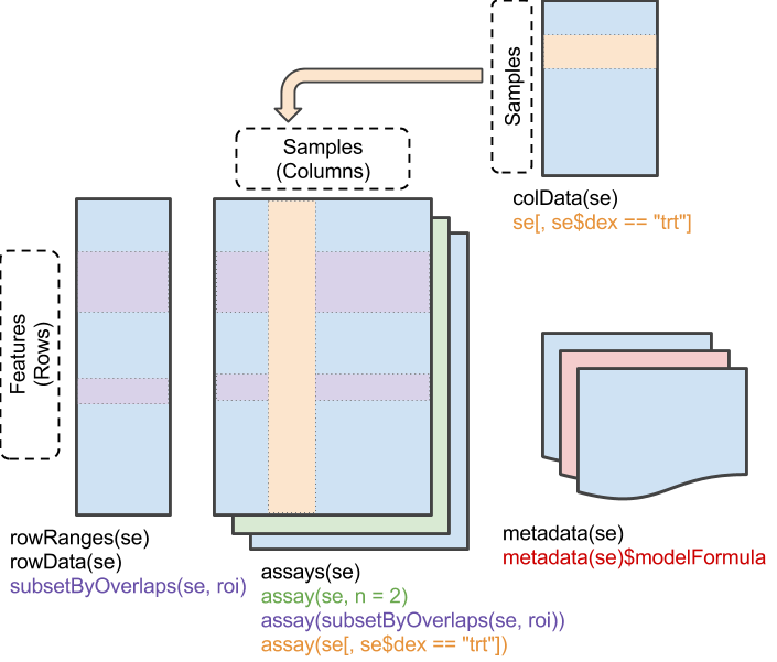
The SummarizedExperiment class is used to store rectangular arrays of experimental results (assays). Although each assay is here drawn as a matrix, higher-dimensional arrays are also supported.

Traditionally, the assay data are stored in-memory as an ordinary array object³³. Storing the data in-memory becomes a real pain with the ever-growing size of ’omics datasets; it is now not uncommon to collect \(10,000-100,000,000\) measurements on \(100 - 1,000,000\) samples, which would occupy \(10-1,000\) gigabytes (GB) if stored in-memory as ordinary R arrays!

Let’s take as an example some single-cell RNA-seq data on 1.3 million brain cells from embryonic mice, generated by 10X Genomics³⁴.

library(TENxBrainData)
# NOTE: This will download the data and may take a little while on the first 
#       run. The result will be cached, however, so subsequent runs are near 
#       instantaneous.
tenx <- TENxBrainData()
# The data are stored in a SingleCellExperiment, an extension of the 
# SummarizedExperiment class.
class(tenx)
#> [1] "SingleCellExperiment"
#> attr(,"package")
#> [1] "SingleCellExperiment"
dim(tenx)
#> [1]   27998 1306127

# How big much memory do the counts data use?
counts <- assay(tenx, "counts", withDimnames = FALSE)
print(object.size(counts))
#> 2144 bytes

The counts data only require a tiny amount of RAM despite it having 27998 rows and 1306127 columns. And the counts object still “feels” like an ordinary R matrix:

# Oooh, pretty-printing.
counts
#> <27998 x 1306127> HDF5Matrix object of type "integer":
#>                [,1]       [,2]       [,3]       [,4] ... [,1306124]
#>     [1,]          0          0          0          0   .          0
#>     [2,]          0          0          0          0   .          0
#>     [3,]          0          0          0          0   .          0
#>     [4,]          0          0          0          0   .          0
#>     [5,]          0          0          0          0   .          0
#>      ...          .          .          .          .   .          .
#> [27994,]          0          0          0          0   .          0
#> [27995,]          1          0          0          2   .          0
#> [27996,]          0          0          0          0   .          0
#> [27997,]          0          0          0          0   .          0
#> [27998,]          0          0          0          0   .          0
#>          [,1306125] [,1306126] [,1306127]
#>     [1,]          0          0          0
#>     [2,]          0          0          0
#>     [3,]          0          0          0
#>     [4,]          0          0          0
#>     [5,]          0          0          0
#>      ...          .          .          .
#> [27994,]          0          0          0
#> [27995,]          1          0          0
#> [27996,]          0          0          0
#> [27997,]          0          0          0
#> [27998,]          0          0          0

# Let's take a subset of the data
counts[1:10, 1:10]
#> <10 x 10> DelayedMatrix object of type "integer":
#>        [,1]  [,2]  [,3]  [,4] ...  [,7]  [,8]  [,9] [,10]
#>  [1,]     0     0     0     0   .     0     0     0     0
#>  [2,]     0     0     0     0   .     0     0     0     0
#>  [3,]     0     0     0     0   .     0     0     0     0
#>  [4,]     0     0     0     0   .     0     0     0     0
#>  [5,]     0     0     0     0   .     0     0     0     0
#>  [6,]     0     0     0     0   .     0     0     0     0
#>  [7,]     0     0     0     0   .     0     0     0     0
#>  [8,]     0     0     0     0   .     2     0     1     1
#>  [9,]     0     0     1     0   .     0     0     0     0
#> [10,]     0     0     0     0   .     0     0     0     0

# Let's compute column sums (crude library sizes) for the first 100 samples.
# TODO: DelayedArray:: prefix shouldn't be necessary
DelayedArray::colSums(counts[, 1:100])
#>   [1]  4046  2087  4654  3193  8444 11178  2375  3672  3115  4592  7899
#>  [12]  5474  2894  5887  8349  7310  3340 23410  7326  3446  4601  5921
#>  [23]  4746  3063  3879  3582  2854  4053  6987  9155  3747  1534  6632
#>  [34]  4099  2846  5025  6688  3742  2982  1998  1808  3121 10561  3874
#>  [45]  4143  1500  2280  3060  4325  3161  2522  1979  6033  3721  2546
#>  [56]  6317  2756  3896  4475  5580  1879  8746  4873  2202  4517  2815
#>  [67]  3809  2580  4655  3523  4717  6436  2434  5704  2962 11654  4848
#>  [78]  5288  6689  5761 11539 15745  2986  2736  3666  2476  2251  3052
#>  [89]  5480  1721  4166  4451  1893  5606  2551  2810  1555  1840  2972
#> [100]  2404

The reason for the small memory footprint and matrix-like “feel” of the counts object is because the counts data are in fact stored on-disk in a Hierarchical Data Format (HDF5) file and we are interacting with the data via the DelayedArray framework.

15.2.1 Discussion

TODO: Make these ‘discussions/challenges’ into a boxes that visually break out

• Talk with your neighbour about the sorts of ‘big data’ you are analysing, the challenges you’ve faced, and strategies you’re using to tackle this.
• TODO: (keep this?) Play around with the tenx and counts data. Could use this to demonstrate the upcoming challenges of chunking (e.g., compute row-wise summary).

TABLE gives some examples of contemporary experiments and the memory requirements if these data are to be stored in-memory as ordinary R arrays.

Assay	Size	nrow	ncol	Number of assays	Type	Reference
WGBS (mCG)	67.992 GB	29,307,073	145	3	2 x dense integer, 1 x dense double	eGTEx (unpublished)
scRNA-seq	146.276 GB	27,998	1,306,127	1	sparse integer	https://bioconductor.org/packages/TENxBrainData/

There are various strategies for handling such large data in R. For example, we could use:

1. Sparse matrices for single-cell RNA-seq data.
2. Run length encoded vectors for ChIP-seq coverage profiles.
3. Storing data on disk, and only bringing into memory as required, for whole genome methylation data³⁵.

Each of these approaches has its strengths, as well as weaknesses and idiosyncrasies. For example,

• Matrix doesn’t support long vectors
• Sparsity is readily lost (e.g., normalization often destroys it)
• etc.

TODO: Lead discussion of limitations

15.2.2 Why learn DelayedArray?

The high-level goals of the DelayedArray framework are:

• Provide a common R interface to array-like data, where the data may be in-memory or on-disk.
• Support delayed operations, which avoid doing any computation until the result is required.
• Support block-processing of the data, which enables bounded-memory and parallel computations.

From the DelayedArray DESCRIPTION:

TODO: Use desc to extract Description field?

Wrapping an array-like object (typically an on-disk object) in a DelayedArray object allows one to perform common array operations on it without loading the object in memory. In order to reduce memory usage and optimize performance, operations on the object are either delayed or executed using a block processing mechanism. Note that this also works on in-memory array-like objects like DataFrame objects (typically with Rle columns), Matrix objects, and ordinary arrays and data frames. (https://bioconductor.org/packages/release/bioc/html/DelayedArray.html)

These goals are similar to that of the tibble and dplyr packages:

A tibble, or tbl_df, is a modern reimagining of the data.frame, keeping what time has proven to be effective, and throwing out what is not. Tibbles are data.frames that are lazy and surly (http://tibble.tidyverse.org/#overview)

dplyr is designed to abstract over how the data is stored. That means as well as working with local data frames, you can also work with remote database tables, using exactly the same R code. (https://dplyr.tidyverse.org/#overview)

An important feature of the DelayedArray framework is that it supports all these strategies, and more, with a common interface that aims to feel like the interface to ordinary arrays, which provides familiarity to R users.

15.2.2.1 Learning goal

• Identify when it is useful to use a DelayedArray instead of an ordinary array or other array-like data structure.

15.3 Overview of DelayedArray framework

The core of DelayedArray framework is implemented in the DelayedArray Bioconductor package. Other packages extend the framework or simply use it as is to enable analyses of large datasets.

15.3.1 The DelayedArray package

The DelayedArray package defines the key classes, generics, and methods³⁶, as well as miscellaneous helper functions, that implement the DelayedArray framework.

The reverse dependencies of DelayedArray are shown below:

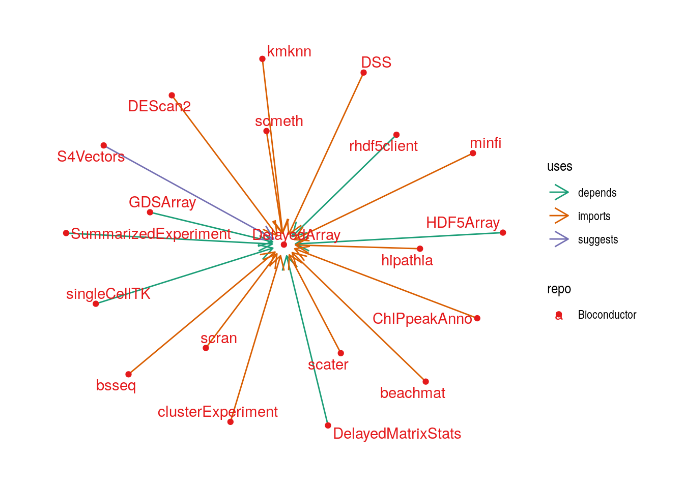
The above figures includes packages that extend the DelayedArray framework in various ways, as well as those that simply use the DelayedArray framework to analyse specific types of ’omics data. We briefly discuss some of these:

15.3.1.1 Packages that extend DelayedArray

There are two ways a package may extend the DelayedArray framework. The first kind of package adds support for a new realization backend (TODO Define?). Examples of this are:

• The HDF5Array package adds the HDF5Array realization backend for accessing and creating data stored on-disk in an HDF5 file. This is typically used for on-disk representation of multidimensional (numeric) arrays.
• The GDSArray package adds the GDSArray backend for accessing and creating data stored on-disk in a GDS file. This is typically used for on-disk representation of genotyping or sequence data.
• The rhdf5client packages adds the H5S_Array realization backend for accessing and creating data stored on a HDF Server, a Python-based web service that can be used to send and receive HDF5 data using an HTTP-based REST interface. This is typically used for on-disk representation of multidimensional (numeric) arrays that need to be shared with multiple users from a central location.

The second kind of package adds methods for computing on DelayedArray instances. Examples of this are:

• The DelayedMatrixStats package provides methods for computing commonly used row- and column-wise summaries of a 2-dimensional DelayedArray.
• The beachmat package provides a consistent C++ class interface for a variety of commonly used matrix types, including ordinary R arrays, sparse matrices, and DelayedArray with various backends.
• The kmknn package provides methods for performing k-means for k-nearest neighbours of data stored in a DelayedArray.
• Packages for performing matrix factorizations, (generalized) linear regression, , etc. (work in progress)

15.3.1.2 Packages that use DelayedArray

• The bsseq package uses the DelayedArray framework to support the analysis of large whole-genome bisulfite methylation sequencing experiments.
• TODO: minfi, scater, scran, others

15.3.2 The DelayedArray class

The DelayedArray class is the key data structure that end users of the DelayedArray framework will interact with. A DelayedMatrix is the same thing as a two-dimensional DelayedArray, just as a matrix is the same thing as a two-dimensional array.

The DelayedArray class has a single slot called the seed. This name is evocative, it is the core of the object.

A package developer may create a subclass of DelayedArray; we will make extensive use of the HDF5Array class, for example.

# TODO: Graphical representation of this network?
# TODO: Illustrate How classes depend on one another
#       a. with DelayedArray as the root
#       b. With DelayedArray as the leaf
showClass(getClass("DelayedArray", where = "DelayedArray"))
#> Class "DelayedArray" [package "DelayedArray"]
#> 
#> Slots:
#>            
#> Name:  seed
#> Class:  ANY
#> 
#> Extends: 
#> Class "DelayedUnaryOp", directly
#> Class "DelayedOp", by class "DelayedUnaryOp", distance 2
#> Class "Array", by class "DelayedUnaryOp", distance 3
#> 
#> Known Subclasses: 
#> Class "DelayedMatrix", directly, with explicit coerce
#> Class "DelayedArray1", directly
#> Class "RleArray", directly
#> Class "RleMatrix", by class "DelayedMatrix", distance 2
showClass(getClass("HDF5Array", where = "HDF5Array"))
#> Class "HDF5Array" [package "HDF5Array"]
#> 
#> Slots:
#>            
#> Name:  seed
#> Class:  ANY
#> 
#> Extends: 
#> Class "DelayedArray", directly
#> Class "DelayedUnaryOp", by class "DelayedArray", distance 2
#> Class "DelayedOp", by class "DelayedArray", distance 3
#> Class "Array", by class "DelayedArray", distance 4
#> 
#> Known Subclasses: 
#> Class "HDF5Matrix", directly, with explicit coerce

15.3.2.1 Learning objectives

In this section, we’ll learn how an end user can construct a DelayedArray from:

• An in-memory array-like object.
• A local, on-disk data store, such as an HDF5 file.
• A remote data store, such as from a HDF Server.

We’ll also learn:

• What defines the “seed contract”
• What types of operations ‘degrade’ an instance of a DelayedArray subclass to a DelayedArray, as well as when and why this matters (TODO Save the when and why it matters to later?).

15.3.2.2 The seed of a DelayedArray

From an end user’s perspective, there are a two broad categories of seed:

1. In-memory seeds
2. Out-of-memory seeds

1. Local, on-disk seeds
2. Remote (in-memory or on-disk) seeds

TODO: Box this out as an aside

For a developer’s perspective, there’s a third category of seed that is defined by the DelayedOp class. Instances of the DelayedOp class are not intended to be manipulated directly by the end user, but they are central to the concept of delayed operations, which we will learn about later (TODO: Link to section).

A seed must implement the “seed contract”³⁷:

• dim(x): Return the dimensions of the seed.
• dimnames(x): Return the (possibly NULL) dimension names of the seed.
• extract_array(x, index): Return a slice, specified by index, of the seed as an ordinary R array.

15.3.2.3 In-memory seeds

To begin, we’ll consider a DelayedArray instance with the simplest seed, an in-memory array:

library(DelayedArray)

mat <- matrix(rep(1:20, 1:20), ncol = 2)
da_mat <- DelayedArray(seed = mat) 
da_mat
#> <105 x 2> DelayedMatrix object of type "integer":
#>        [,1] [,2]
#>   [1,]    1   15
#>   [2,]    2   15
#>   [3,]    2   15
#>   [4,]    3   15
#>   [5,]    3   15
#>    ...    .    .
#> [101,]   14   20
#> [102,]   14   20
#> [103,]   14   20
#> [104,]   14   20
#> [105,]   14   20

We can use other, more complex, array-like objects as the seed, such as Matrix objects from the Matrix package:

library(Matrix)
Mat <- Matrix(mat)
da_Mat <- DelayedArray(seed = Mat)
# NOTE: The type is "double" because of how the Matrix package stores the data.
da_Mat
#> <105 x 2> DelayedMatrix object of type "double":
#>        [,1] [,2]
#>   [1,]    1   15
#>   [2,]    2   15
#>   [3,]    2   15
#>   [4,]    3   15
#>   [5,]    3   15
#>    ...    .    .
#> [101,]   14   20
#> [102,]   14   20
#> [103,]   14   20
#> [104,]   14   20
#> [105,]   14   20

We can even use data frames as the seed of a two-dimensional DelayedArray.

df <- as.data.frame(mat)
da_df <- DelayedArray(seed = df)
# NOTE: This inherits the (default) column names of the data.frame.
da_df
#> <105 x 2> DelayedMatrix object of type "integer":
#>     V1 V2
#>   1  1 15
#>   2  2 15
#>   3  2 15
#>   4  3 15
#>   5  3 15
#> ...  .  .
#> 101 14 20
#> 102 14 20
#> 103 14 20
#> 104 14 20
#> 105 14 20

library(tibble)
tbl <- as_tibble(mat)
da_tbl <- DelayedArray(seed = tbl)
# NOTE: This inherits the (default) column names of the tibble.
da_tbl
#> <105 x 2> DelayedMatrix object of type "integer":
#>     V1 V2
#>   1  1 15
#>   2  2 15
#>   3  2 15
#>   4  3 15
#>   5  3 15
#> ...  .  .
#> 101 14 20
#> 102 14 20
#> 103 14 20
#> 104 14 20
#> 105 14 20

DF <- as(mat, "DataFrame")
da_DF <- DelayedArray(seed = DF)
# NOTE: This inherits the (default) column names of the DataFrame.
da_DF
#> <105 x 2> DelayedMatrix object of type "integer":
#>        V1 V2
#>   [1,]  1 15
#>   [2,]  2 15
#>   [3,]  2 15
#>   [4,]  3 15
#>   [5,]  3 15
#>    ...  .  .
#> [101,] 14 20
#> [102,] 14 20
#> [103,] 14 20
#> [104,] 14 20
#> [105,] 14 20

A package developer can also implement a novel in-memory seed. For example, the DelayedArray package defines the RleArraySeed class³⁸. This can be used as the seed of an RleArray, a DelayedArray subclass for storing run-length encoded data.

# NOTE: The DelayedArray package does not expose the RleArraySeed() constructor.
#       Instead, we directly call the RleArray() constructor on the run-length 
#       encoded data.
da_Rle <- RleArray(rle = Rle(mat), dim = dim(mat))
da_Rle
#> <105 x 2> RleMatrix object of type "integer":
#>        [,1] [,2]
#>   [1,]    1   15
#>   [2,]    2   15
#>   [3,]    2   15
#>   [4,]    3   15
#>   [5,]    3   15
#>    ...    .    .
#> [101,]   14   20
#> [102,]   14   20
#> [103,]   14   20
#> [104,]   14   20
#> [105,]   14   20

The RleArray examples illustrates some important concepts in the DelayedArray class hierarchy that warrants reiteration and expansion.

15.3.2.4 Degrading DelayedArray subclasses

The da_Rle object is an RleMatrix, a direct subclass of RleArray and a direct subclass of DelayedMatrix. Both RleArray and DelayedMatrix are direct subclasses of a DelayedArray. As such, in accordance with properties of S4 class inheritance, an RleMatrix is a DelayedArray.

da_Rle
#> <105 x 2> RleMatrix object of type "integer":
#>        [,1] [,2]
#>   [1,]    1   15
#>   [2,]    2   15
#>   [3,]    2   15
#>   [4,]    3   15
#>   [5,]    3   15
#>    ...    .    .
#> [101,]   14   20
#> [102,]   14   20
#> [103,]   14   20
#> [104,]   14   20
#> [105,]   14   20
is(da_Rle, "DelayedArray")
#> [1] TRUE
showClass(getClass("RleMatrix", where = "DelayedArray"))
#> Class "RleMatrix" [package "DelayedArray"]
#> 
#> Slots:
#>            
#> Name:  seed
#> Class:  ANY
#> 
#> Extends: 
#> Class "DelayedMatrix", directly
#> Class "RleArray", directly
#> Class "DelayedArray", by class "DelayedMatrix", distance 2
#> Class "DelayedUnaryOp", by class "DelayedMatrix", distance 2
#> Class "DelayedOp", by class "DelayedMatrix", distance 2
#> Class "Array", by class "DelayedMatrix", distance 2
#> Class "DataTable", by class "DelayedMatrix", distance 2
#> Class "DataTable_OR_NULL", by class "DelayedMatrix", distance 3

However, if we do (almost) anything to the RleMatrix, the result is ‘degraded’ to a DelayedMatrix. This ‘degradation’ isn’t an issue in and of itself, but it can be surprising and can complicate writing functions that expect a certain type of input (e.g., S4 methods).

# NOTE: Adding one to each element will 'degrade' the result.
da_Rle + 1L
#> <105 x 2> DelayedMatrix object of type "integer":
#>        [,1] [,2]
#>   [1,]    2   16
#>   [2,]    3   16
#>   [3,]    3   16
#>   [4,]    4   16
#>   [5,]    4   16
#>    ...    .    .
#> [101,]   15   21
#> [102,]   15   21
#> [103,]   15   21
#> [104,]   15   21
#> [105,]   15   21
is(da_Rle + 1L, "RleMatrix")
#> [1] FALSE

# NOTE: Subsetting will 'degrade' the result.
da_Rle[1:10, ]
#> <10 x 2> DelayedMatrix object of type "integer":
#>       [,1] [,2]
#>  [1,]    1   15
#>  [2,]    2   15
#>  [3,]    2   15
#>  [4,]    3   15
#>  [5,]    3   15
#>  [6,]    3   15
#>  [7,]    4   15
#>  [8,]    4   15
#>  [9,]    4   15
#> [10,]    4   15
is(da_Rle[1:10, ], "RleMatrix")
#> [1] FALSE

# NOTE: Changing the dimnames will 'degrade' the result.
da_Rle_with_dimnames <- da_Rle
colnames(da_Rle_with_dimnames) <- c("A", "B")
da_Rle_with_dimnames
#> <105 x 2> DelayedMatrix object of type "integer":
#>         A  B
#>   [1,]  1 15
#>   [2,]  2 15
#>   [3,]  2 15
#>   [4,]  3 15
#>   [5,]  3 15
#>    ...  .  .
#> [101,] 14 20
#> [102,] 14 20
#> [103,] 14 20
#> [104,] 14 20
#> [105,] 14 20
is(da_Rle_with_dimnames, "RleMatrix")
#> [1] FALSE

# NOTE: Transposing will 'degrade' the result.
t(da_Rle)
#> <2 x 105> DelayedMatrix object of type "integer":
#>        [,1]   [,2]   [,3]   [,4] ... [,102] [,103] [,104] [,105]
#> [1,]      1      2      2      3   .     14     14     14     14
#> [2,]     15     15     15     15   .     20     20     20     20
is(t(da_Rle), "RleMatrix")
#> [1] FALSE

# NOTE: Even adding zero (conceptually a no-op) will 'degrade' the result.
da_Rle + 0L
#> <105 x 2> DelayedMatrix object of type "integer":
#>        [,1] [,2]
#>   [1,]    1   15
#>   [2,]    2   15
#>   [3,]    2   15
#>   [4,]    3   15
#>   [5,]    3   15
#>    ...    .    .
#> [101,]   14   20
#> [102,]   14   20
#> [103,]   14   20
#> [104,]   14   20
#> [105,]   14   20

There are some exceptions to this rule, when the DelayedArray framework can recognise/guarantee that the operation is a no-op that will leave the object in its current state:

# NOTE: Subsetting to select the entire object does not 'degrade' the result.
da_Rle[seq_len(nrow(da_Rle)), seq_len(ncol(da_Rle))]
#> <105 x 2> RleMatrix object of type "integer":
#>        [,1] [,2]
#>   [1,]    1   15
#>   [2,]    2   15
#>   [3,]    2   15
#>   [4,]    3   15
#>   [5,]    3   15
#>    ...    .    .
#> [101,]   14   20
#> [102,]   14   20
#> [103,]   14   20
#> [104,]   14   20
#> [105,]   14   20
is(da_Rle[seq_len(nrow(da_Rle)), seq_len(ncol(da_Rle))], "RleMatrix")
#> [1] TRUE

# NOTE: Transposing and transposing back does not 'degrade' the result.
t(t(da_Rle))
#> <105 x 2> RleMatrix object of type "integer":
#>        [,1] [,2]
#>   [1,]    1   15
#>   [2,]    2   15
#>   [3,]    2   15
#>   [4,]    3   15
#>   [5,]    3   15
#>    ...    .    .
#> [101,]   14   20
#> [102,]   14   20
#> [103,]   14   20
#> [104,]   14   20
#> [105,]   14   20
is(t(t(da_Rle)), "RleMatrix")
#> [1] TRUE

A particularly important example of this ‘degrading’ to be aware of is when accessing the assays of a SummarizedExperiment via the assay() and assays() getters. Each of these getters has an argument withDimnames with a default value of TRUE; this copies the dimnames of the SummarizedExperiment to the returned assay. Consequently, this may ‘degrade’ the object(s) returned by assay() and assays() to DelayedArray. To avoid this, use withDimnames = FALSE in the call to assay() and assays().

library(SummarizedExperiment)
# Construct a SummarizedExperiment with column names 'A' and 'B' and da_Rle as 
# the assay data.
se <- SummarizedExperiment(da_Rle, colData = DataFrame(row.names = c("A", "B")))
se
#> class: SummarizedExperiment 
#> dim: 105 2 
#> metadata(0):
#> assays(1): ''
#> rownames: NULL
#> rowData names(0):
#> colnames(2): A B
#> colData names(0):

# NOTE: dimnames are copied, so the result is 'degraded'.
assay(se)
#> <105 x 2> DelayedMatrix object of type "integer":
#>         A  B
#>   [1,]  1 15
#>   [2,]  2 15
#>   [3,]  2 15
#>   [4,]  3 15
#>   [5,]  3 15
#>    ...  .  .
#> [101,] 14 20
#> [102,] 14 20
#> [103,] 14 20
#> [104,] 14 20
#> [105,] 14 20
is(assay(se), "RleMatrix")
#> [1] FALSE

# NOTE: dimnames are not copied, so the result is not 'degraded'.
assay(se, withDimnames = FALSE)
#> <105 x 2> RleMatrix object of type "integer":
#>        [,1] [,2]
#>   [1,]    1   15
#>   [2,]    2   15
#>   [3,]    2   15
#>   [4,]    3   15
#>   [5,]    3   15
#>    ...    .    .
#> [101,]   14   20
#> [102,]   14   20
#> [103,]   14   20
#> [104,]   14   20
#> [105,]   14   20
is(assay(se, withDimnames = FALSE), "RleMatrix")
#> [1] TRUE

As noted up front, the degradation isn’t in and of itself a problem. However, if you are passing an object to a function that expects an RleMatrix, for example, some care needs to be taken to ensure that the object isn’t accidentally ‘degraded’ along the way to a DelayedMatrix.

To summarise, the lessons here are:

• Modifying an instance of a DelayedArray subclass will almost always ‘degrade’ it to a DelayedArray.
• It is very easy to accidentally trigger this ‘degradation’.
• This ‘degradation’ can complicate method dispatch.

15.3.2.5 Out-of-memory seeds

The DelayedArray framework really shines when working with out-of-memory seeds. It can give the user the “feel” of interacting with an ordinary R array but allows for the data to be stored on a local disk or even on a remote server, thus reducing (local) memory usage.

15.3.2.5.1 Local on-disk seeds

The HDF5Array package defines the HDF5Array class, a DelayedArray subclass for data stored on disk in a HDF5 file. The seed of an HDF5Array is a HDF5ArraySeed. It is important to note that creating a HDF5Array does not read the data into memory! The data remain on disk until requested (we’ll see how to do this later on in the workshop).

library(HDF5Array)

hdf5_file <- file.path(
    "500_Effectively_Using_the_DelayedArray_Framework", 
    "hdf5_mat.h5")
# NOTE: We can use rhdf5::h5ls() to take a look what is in the HDF5 file.
#       This is very useful when working interactively!
rhdf5::h5ls(hdf5_file)
#>   group     name       otype  dclass  dim
#> 0     / hdf5_mat H5I_DATASET INTEGER  x 2

# We can create the HDF5Array by first creating a HDF5ArraySeed and then 
# creating the HDF5Array.
hdf5_seed <- HDF5ArraySeed(filepath = hdf5_file, name = "hdf5_mat")
da_hdf5 <- DelayedArray(seed = hdf5_seed)
da_hdf5
#> <105 x 2> HDF5Matrix object of type "integer":
#>        [,1] [,2]
#>   [1,]    1   15
#>   [2,]    2   15
#>   [3,]    2   15
#>   [4,]    3   15
#>   [5,]    3   15
#>    ...    .    .
#> [101,]   14   20
#> [102,]   14   20
#> [103,]   14   20
#> [104,]   14   20
#> [105,]   14   20

# Alternatively, we can create this in one go using the HDF5Array() constructor.    
da_hdf5 <- HDF5Array(filepath = hdf5_file, name = "hdf5_mat")
da_hdf5
#> <105 x 2> HDF5Matrix object of type "integer":
#>        [,1] [,2]
#>   [1,]    1   15
#>   [2,]    2   15
#>   [3,]    2   15
#>   [4,]    3   15
#>   [5,]    3   15
#>    ...    .    .
#> [101,]   14   20
#> [102,]   14   20
#> [103,]   14   20
#> [104,]   14   20
#> [105,]   14   20

Other on-disk seeds are possible such as fst, bigmemory, ff, or matter.

15.3.2.5.2 Remote seeds

The rhdf5client packages defines the H5S_Array class, a DelayedArray subclass for data stored on a remote HDF Server. The seed of an H5S_Array is a H5S_ArraySeed. It is important to note that creating a H5S_Array does not read the data into memory! The data remain on the server until requested.

library(rhdf5client)
#> 
#> Attaching package: 'rhdf5client'
#> The following object is masked from 'package:tidygraph':
#> 
#>     groups
da_h5s <- HSDS_Matrix(URL_hsds(), "/home/stvjc/hdf5_mat.h5")
da_h5s
#> <105 x 2> H5S_Matrix object of type "double":
#>        [,1] [,2]
#>   [1,]    1   15
#>   [2,]    2   15
#>   [3,]    2   15
#>   [4,]    3   15
#>   [5,]    3   15
#>    ...    .    .
#> [101,]   14   20
#> [102,]   14   20
#> [103,]   14   20
#> [104,]   14   20
#> [105,]   14   20

15.3.2.6 So what seed should I use?

Notably, da_mat, da_Mat, da_tbl, da_df, da_Rle, da_hdf5, and da_h5s all “look” and “feel” much the same. The DelayedArray is a very light wrapper around the seed that formalises this consistent “look” and “feel”.

If your data always fit in memory, and it’s still comfortable to work with it interactively, then you should probably stick with using ordinary matrix and array objects. If, however, your data sometimes don’t fit in memory or it becomes painful to work with them when they are in-memory, you should consider a disk-backed DelayedArray. If you need to share a large dataset with a number of uses, and most users only need slices of it, you may want to consider a remote server-backed DelayedArray.

Not suprisingly, working with in-memory seeds will typically be faster than disk-backed or remote seeds; you are trading off memory-usage and data access times to obtain faster performance.

Below are some further opinionated recommendations.

Although the DelayedArray is a light wrapper, it does introduce some overhead. For example, operations on a DelayedArray with an array or Matrix seed will be slower than operating on the array or Matrix directly. For some operations this is almost non-existant (e.g., seed-aware operations in the DelayedMatrixStats package), but for others this overhead may be noticeable. Conversely, a potential upside to wrapping a Matrix in a DelayedArray is that it can now leverage the block-processing strategy of the DelayedArray framework.

If you need a disk-backed DelayedArray, I would recommend using HDF5Array as the backend at this time. HDF5 is a well-established scientific data format and the HDF5Array package is developed by the core Bioconductor team. Furthermore, several bioinformatics tools natively export HDF5 files (e.g., kallisto, CellRanger from 10x Genomics). One potential downside of HDF5 is the recent split into “Community” and “Enterprise Support” editions. It’s not yet clear how this will affect the HDF5 library or its community. Other on-disk backends may not yet have well-established formats or libraries (e.g., TileDB). A topic of on-going research in the Bioconductor community is to compare the performance of HDF5 to other disk-backed data stores. Another topic is how to best choose the layout of the data on disk, often referred to as the “chunking” of the data. For example, if the data is stored in column-major order then it might be expected that row-wise data access suffers.

One final comment. If you are trying to support both in-memory and on-disk data, it may be worth considering using DelayedArray for everything rather than trying to support both DelayedArray and ordinary arrays. This is particularly true for internal, non-user facing code. Otherwise your software may need separate code paths for array and DelayedArray inputs, although the need for separate branches is reducing. For example, when I initially added support for the DelayedArray framework in bsseq (~2 years ago), I opted to remove support for ordinary arrays. However, more recently I added support for the DelayedArray framework in minfi, and there I opted to maintain support for ordinary arrays. I’ve found that as the DelayedArray framework matures and expands, it is increasingly common that the same code “just works” for both array and DelayedArray objects. Maintaining support for ordinary arrays can also be critical for popular Bioconductor packages, although this can be handled by having functions that accept an array as input simply wrapping them in a DelayedArray for internal computations.

15.3.3 Operating on DelayedArray objects

Now that we know what a DelayedArray is, it’s various subclasses, and how to construct these, we will discuss how to use operate on DelayedArray objects.

We’ll cover three fundamental concepts:

1. Delayed operations
2. Block-processing
3. Realization

These three concepts work hand-in-hand. Delayed operations are exactly that, the operation is recorded but performing the operation is delayed until the result is required; realization is the process of executing the delayed operations; and block-processing is used to perform operations, including realization, on blocks of the DelayedArray.

15.3.3.1 Learning goals

• Become familiar with the fundamental concepts of delayed operations, block-processing, and realization.
• TODO Construct a DelayedArray from scratch by writing data to a RealizationSink.

15.3.3.2 Delayed operations

A delayed operation is one that is not actually performed until the result is required. Here’s a simple example of a delayed operations: taking the negative of every element of a HDF5Matrix.

da_hdf5
#> <105 x 2> HDF5Matrix object of type "integer":
#>        [,1] [,2]
#>   [1,]    1   15
#>   [2,]    2   15
#>   [3,]    2   15
#>   [4,]    3   15
#>   [5,]    3   15
#>    ...    .    .
#> [101,]   14   20
#> [102,]   14   20
#> [103,]   14   20
#> [104,]   14   20
#> [105,]   14   20
-da_hdf5
#> <105 x 2> DelayedMatrix object of type "integer":
#>        [,1] [,2]
#>   [1,]   -1  -15
#>   [2,]   -2  -15
#>   [3,]   -2  -15
#>   [4,]   -3  -15
#>   [5,]   -3  -15
#>    ...    .    .
#> [101,]  -14  -20
#> [102,]  -14  -20
#> [103,]  -14  -20
#> [104,]  -14  -20
#> [105,]  -14  -20

It may look like running -da_hdf5 has taken the negative of every element. However, we can see this is in fact not the case by using the showtree() function to inspect the internal state of these objects³⁹:

showtree(da_hdf5)
#> 105x2 integer: HDF5Matrix object
#> └─ 105x2 integer: [seed] HDF5ArraySeed object

# NOTE: The "Unary iso op" line is 'recording' the `-` as a delayed operation.
showtree(-da_hdf5)
#> 105x2 integer: DelayedMatrix object
#> └─ 105x2 integer: Unary iso op
#>    └─ 105x2 integer: [seed] HDF5ArraySeed object

To further illustrate the idea, let’s perform some delayed operations on a large HDF5Array and compare them to performing the operations on the equivalent array.

library(h5vcData)

tally_file <- system.file("extdata", "example.tally.hfs5", package = "h5vcData")
x_h5 <- HDF5Array::HDF5Array(tally_file, "/ExampleStudy/16/Coverages")
x_h5
#> <6 x 2 x 90354753> HDF5Array object of type "integer":
#> ,,1
#>      [,1] [,2]
#> [1,]    0    0
#> [2,]    0    0
#>  ...    .    .
#> [5,]    0    0
#> [6,]    0    0
#> 
#> ...
#> 
#> ,,90354753
#>      [,1] [,2]
#> [1,]    0    0
#> [2,]    0    0
#>  ...    .    .
#> [5,]    0    0
#> [6,]    0    0
x <- as.array(x_h5)

# Delayed operations are fast compared to ordinary operations! 
system.time(x_h5 + 100L) 
#>    user  system elapsed 
#>   0.008   0.000   0.005
system.time(x + 100L) 
#>    user  system elapsed 
#>   2.672   1.356   4.026

# Delayed operations can be chained
system.time(t(x_h5[1, , 1:100] + 100L))
#>    user  system elapsed 
#>   0.016   0.000   0.018

Rather than modifying the data stored in the HDF5 file, which can be costly for large datasets, we’ve recorded the ‘idea’ of these operations as a tree of DelayedOp objects. Each node in the tree is represented by a DelayedOp object, of which there are 6 concrete subclasses:

Node type	Out-degree	Operation
DelayedSubset	1	Multi-dimensional single bracket subsetting
DelayedAperm	1	Extended aperm() (can drop dimensions)
DelayedUnaryIsoOp	1	Unary op that preserves the geometry (e.g., -, log())
DelayedDimnames	1	Set dimnames
DelayedNaryIsoOp	N	N-ary op that preserves the geometry
DelayedAbind	N	abind()

15.3.3.3 Block-processing

Block-processing allows you to iterate over blocks of a DelayedArray in a manner that abstracts over the backend.

The following cartoon illustrates the basic idea of block-processing:

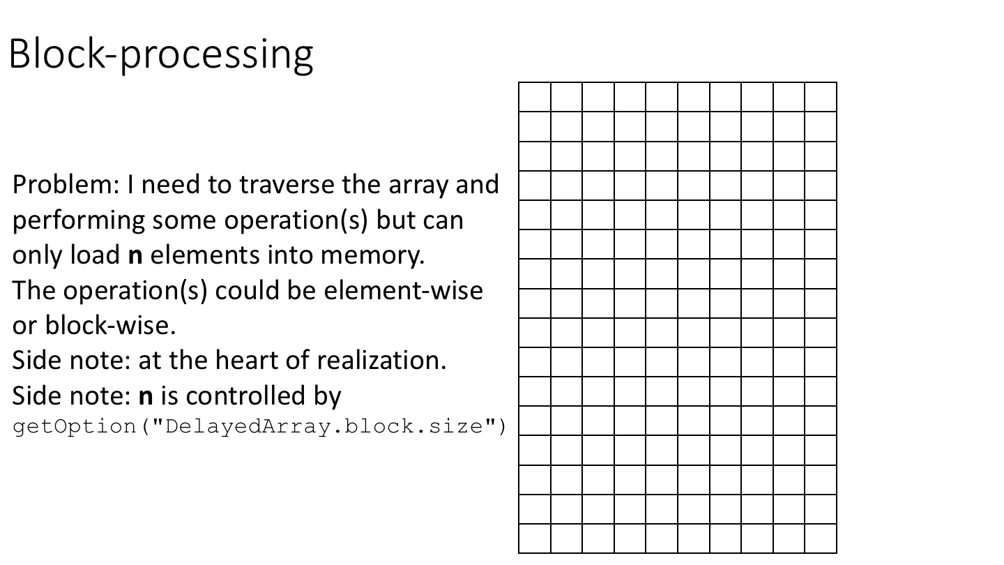
To implement block-processing, we first construct an ArrayGrid over the DelayedArray. Each element of the ArrayGrid is called an ArrayViewport. We iterate over the ArrayGrid, extract the corresponding ArrayViewport, and load the data for that block into memory as an ordinary R array where it can be processed using ordinary R functions.

In pseudocode, we might implement block processing as follows:

# Construct an ArrayGrid over 'x'. 
# NOTE: blockGrid() is explained below.
grid <- blockGrid(x)
for (b in seq_along(grid)) {
    # Construct an ArrayViewPort using the b-th element of the ArrayGrid.
    viewport <- grid[[b]]
    # Read the block of data using the current 'viewport' applied to 'x'.
    block <- read_block(x, viewport)
    # Apply our function to 'block' (which is an ordinary R array).
    FUN(block)
}

In practice, when constructing the ArrayGrid for a particular operation, we need to consider a few issues:

1. Constraints on how much data we can bring into memory (the ‘maximum block length’).
2. The geometry of the ArrayGrid, which will control the order in which we access elements.
3. How the data are physically stored (‘chunking’ of the data on disk).

15.3.3.3.1 Maximum block length

There is a global option getOption("DelayedArray.block.size") for controlling how much data is brough into memory with default value corresponding to each block containing a maximum of 45 Mb of data. It’s good practice to respect this value, however, some algorithms may require this be ignored (e.g., if you require a full column’s worth of data for each block).

15.3.3.3.2 Chunking and data structure

Regardless of the backend, the data will be stored with a particular structure. For example, ordinary R arrays store the data in column-major order. The geometry of the data structure is especially relevant for HDF5 files.

The HDF5 format supports ‘chunking’ of data to maximize data access performance. From https://support.hdfgroup.org/HDF5/doc/Advanced/Chunking/index.html:

Datasets in HDF5 can represent arrays with any number of dimensions (up to 32). However, in the file this dataset must be stored as part of the 1-dimensional stream of data that is the low-level file. The way in which the multidimensional dataset is mapped to the serial file is called the layout. The most obvious way to accomplish this is to simply flatten the dataset in a way similar to how arrays are stored in memory, serializing the entire dataset into a monolithic block on disk, which maps directly to a memory buffer the size of the dataset. This is called a contiguous layout.

An alternative to the contiguous layout is the chunked layout. Whereas contiguous datasets are stored in a single block in the file, chunked datasets are split into multiple chunks which are all stored separately in the file. The chunks can be stored in any order and any position within the HDF5 file. Chunks can then be read and written individually, improving performance when operating on a subset of the dataset.

Although this sounds similar to the blocks used in block-processing, the two are distinct.

Chunks are used to determine how the data are stored, blocks are used to determine how the data are accessed via the ArrayGrid. That is, you can use a different ArrayGrid geometry to the chunk geometry, but performance may be suboptimal.

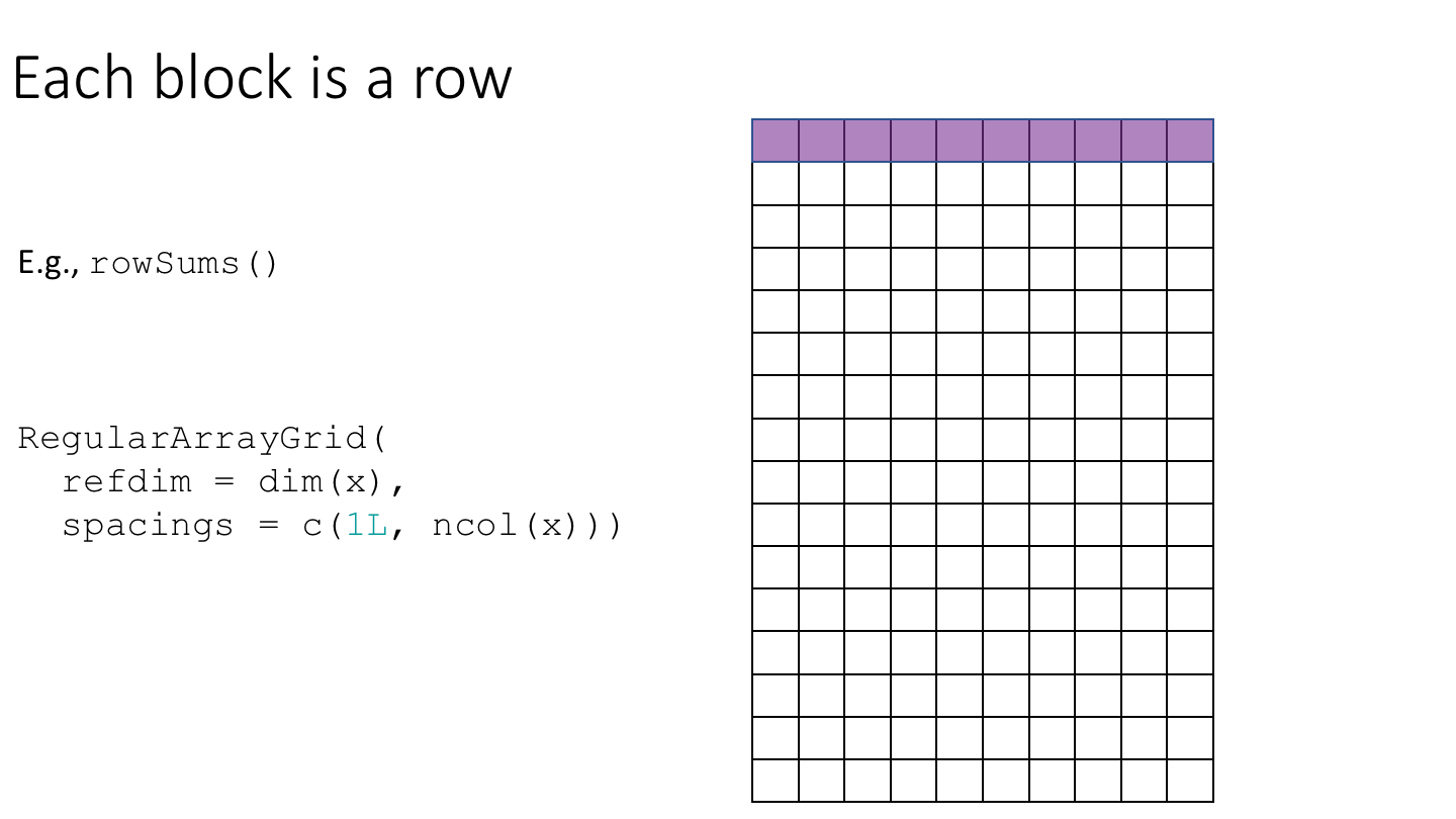
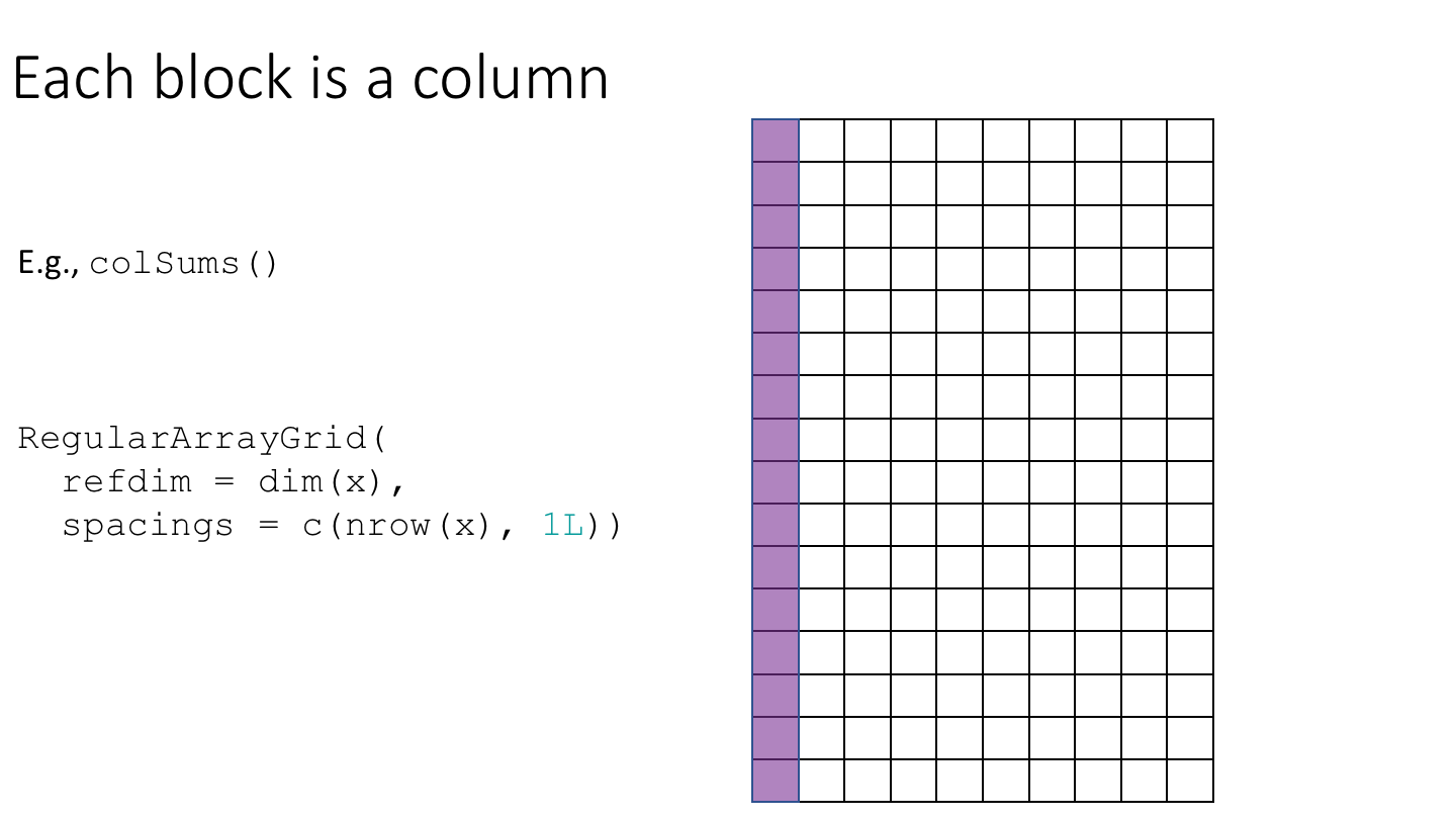
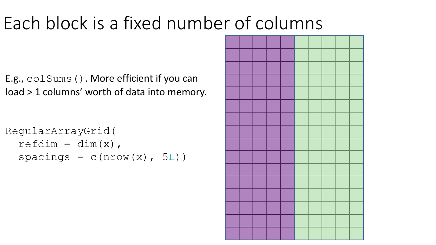
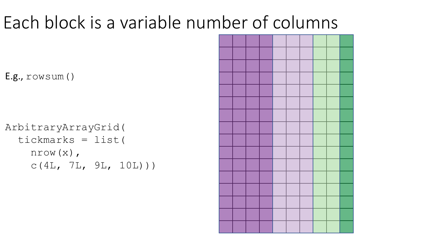
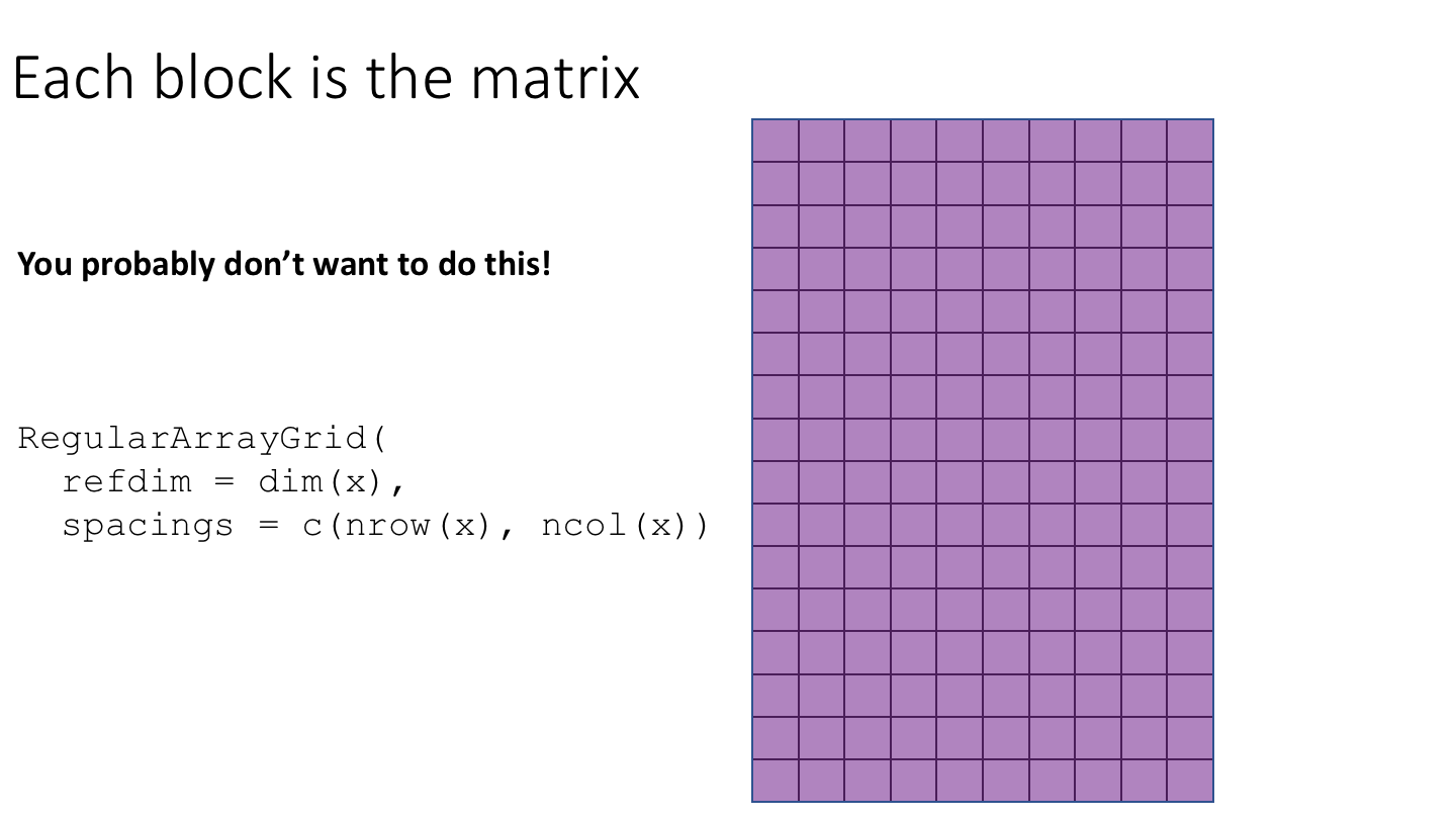
15.3.3.3.3 Geometry of the ArrayGrid

The ArrayGrid could be a regularly spaced grid (a RegularArrayGrid) or a grid with arbitrary spacing (an ArbitraryArrayGrid).

The DelayedArray package includes some helper functions for setting up ArrayGrid instances with particular geometries and other properties.

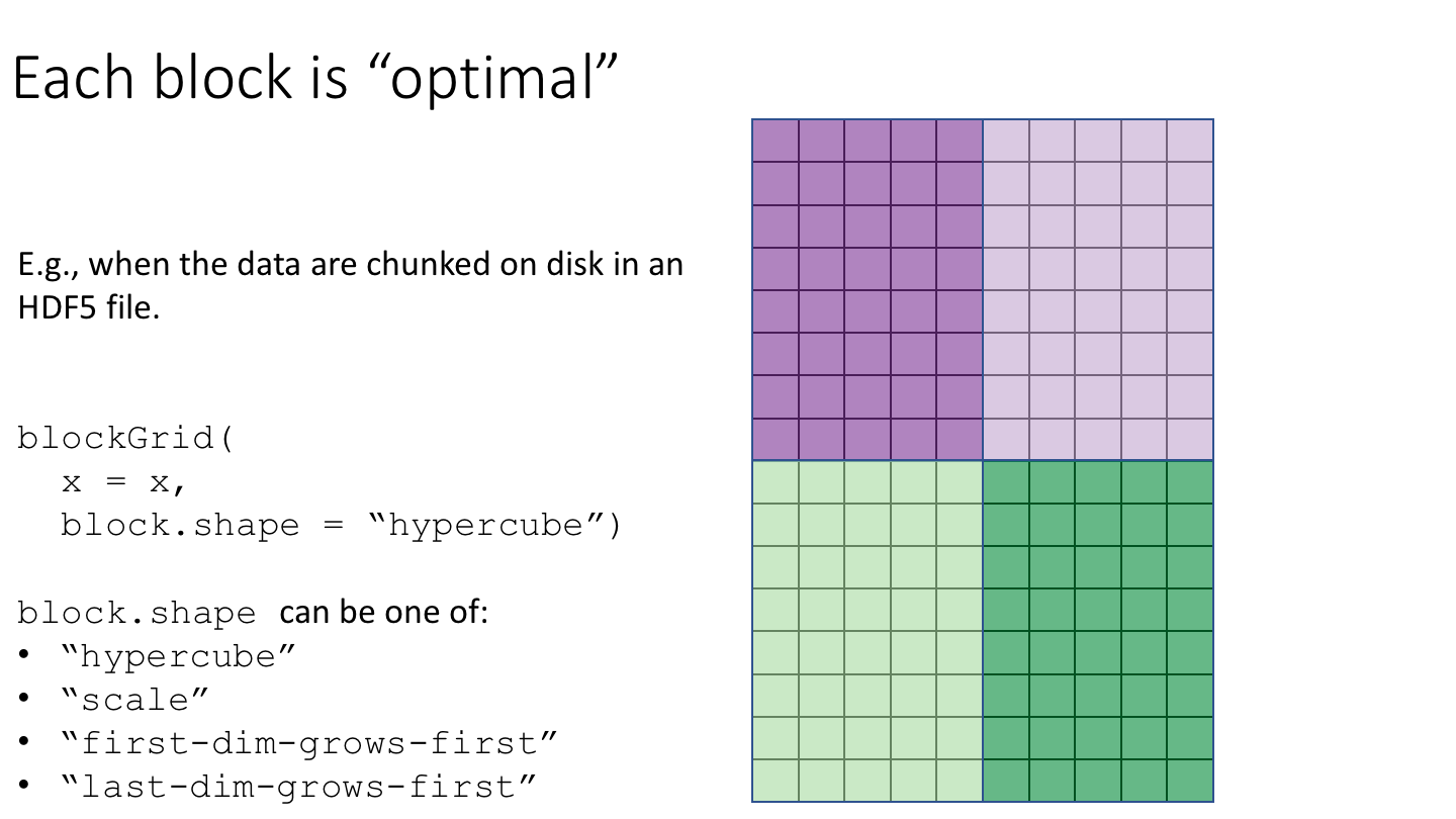
The blockGrid() function returns the “optimal” ArrayGrid for block-processing. The grid is “optimal” in the sense that:

• It’s “compatible” with the chunk grid (i.e. with chunkGrid(x) or with the chunk grid supplied via the chunk.grid argument). That is, the chunks are contained in the blocks. In other words, chunks never cross block boundaries.
• Its “resolution” is such that the blocks have a length that is as close as possible to (but does not exceed) block.maxlength. An exception is when some chunks are already >= block.maxlength, in which case the returned grid is the same as the chunk grid.

15.3.3.3.4 Block-processing in practice

In practice, most block-processing algorithms can be implemented by constructing an ArrayGrid with a suitable geometry and then using DelayedArray::blockApply() or DelayedArray::blockReduce().

As an example, let’s compute row and column medians of da_hdf5. We’ll start by constructing ArrayGrid instances over the rows and columns of da_hdf5.

# NOTE: Making block-processing verbose to show what's going on under the hood.
DelayedArray:::set_verbose_block_processing(TRUE)
#> [1] FALSE
system.time(
    row_medians <- blockApply(
        x = da_hdf5, 
        FUN = median, 
        grid = RegularArrayGrid(
            refdim = dim(da_hdf5),
            spacings = c(1L, ncol(da_hdf5)))))
#>    user  system elapsed 
#>   0.128   1.308   1.737
head(row_medians)
#> [[1]]
#> [1] 8
#> 
#> [[2]]
#> [1] 8.5
#> 
#> [[3]]
#> [1] 8.5
#> 
#> [[4]]
#> [1] 9
#> 
#> [[5]]
#> [1] 9
#> 
#> [[6]]
#> [1] 9
system.time(
    col_medians <- blockApply(
        x = da_hdf5, 
        FUN = median, 
        grid = RegularArrayGrid(
            refdim = dim(da_hdf5),
            spacings = c(nrow(da_hdf5), 1L))))
#>    user  system elapsed 
#>   0.056   0.136   0.274
head(col_medians)
#> [[1]]
#> [1] 10
#> 
#> [[2]]
#> [1] 18

That works, but is somewhat slow for computing row maximums because we read from the HDF5 file nrow(da_hdf5) ( 105) times. We would be better off loading multiple rows of data per block. There are several ways to do this; here, we’ll use DelayedArray::blockGrid() to construct an optimal ArrayGrid and matrixStats::rowMedians() and matrixStats::colMedians() to compute the row and column maximums.

system.time(
    row_medians <- blockApply(
        x = da_hdf5, 
        FUN = matrixStats::rowMedians, 
        grid = blockGrid(
            x = da_hdf5,
            block.shape = "first-dim-grows-first")))
#> Processing block 1/1 ... OK
#>    user  system elapsed 
#>    0.02    0.00    0.02
head(row_medians)
#> [[1]]
#>   [1]  8.0  8.5  8.5  9.0  9.0  9.0  9.5  9.5  9.5  9.5 10.0 10.0 10.0 10.0
#>  [15] 10.0 11.0 11.0 11.0 11.0 11.0 11.0 11.5 11.5 11.5 11.5 11.5 11.5 11.5
#>  [29] 12.0 12.0 12.0 12.5 12.5 12.5 12.5 12.5 13.0 13.0 13.0 13.0 13.0 13.0
#>  [43] 13.0 13.0 13.0 13.5 13.5 13.5 14.0 14.0 14.0 14.0 14.0 14.0 14.0 14.5
#>  [57] 14.5 14.5 14.5 14.5 14.5 14.5 14.5 14.5 14.5 14.5 15.5 15.5 15.5 15.5
#>  [71] 15.5 15.5 15.5 15.5 15.5 15.5 15.5 15.5 16.0 16.0 16.0 16.0 16.0 16.0
#>  [85] 16.0 16.5 16.5 16.5 16.5 16.5 16.5 17.0 17.0 17.0 17.0 17.0 17.0 17.0
#>  [99] 17.0 17.0 17.0 17.0 17.0 17.0 17.0
system.time(
    col_medians <- blockApply(
        x = da_hdf5, 
        FUN = matrixStats::colMedians, 
        grid = blockGrid(
            x = da_hdf5,
            block.shape = "last-dim-grows-first")))
#> Processing block 1/1 ... OK
#>    user  system elapsed 
#>   0.020   0.000   0.018
head(col_medians)
#> [[1]]
#> [1] 10 18

For larger problems, we can improve performance by processing blocks in parallel by passing an appropriate BiocParallelParam object via the bpparam argument of blockApply() and blockReduce().

Although blockApply() and blockReduce() cover most of the block-processing tasks, sometimes you may need to implement the block-processing at a lower level. For example, you may need to iterate over multiple DelayedArray objects or your FUN returns an object equally large (or larger) than the block. The details of these abstractions are still being worked out, but some likely candidates include methods that conceptually do:

• blockMapply()
• blockApplyWithRealization()
• blockMapplyWithRealization()

15.3.3.4 Realization

Realization is the process of taking a DelayedArray, executing any delayed operations, and returning the result as a new DelayedArray with the appropriate backend.

Returning to our earlier example with data from the h5vcData package:

x_h5
#> <6 x 2 x 90354753> HDF5Array object of type "integer":
#> ,,1
#>      [,1] [,2]
#> [1,]    0    0
#> [2,]    0    0
#>  ...    .    .
#> [5,]    0    0
#> [6,]    0    0
#> 
#> ...
#> 
#> ,,90354753
#>      [,1] [,2]
#> [1,]    0    0
#> [2,]    0    0
#>  ...    .    .
#> [5,]    0    0
#> [6,]    0    0
showtree(x_h5)
#> 6x2x90354753 integer: HDF5Array object
#> └─ 6x2x90354753 integer: [seed] HDF5ArraySeed object
y <- t(x_h5[1, , 1:10000000] + 100L)
showtree(y)
#> 10000000x2 integer: DelayedMatrix object
#> └─ 10000000x2 integer: Unary iso op
#>    └─ 10000000x2 integer: Aperm (perm=c(3,2))
#>       └─ 1x2x10000000 integer: Subset
#>          └─ 6x2x90354753 integer: [seed] HDF5ArraySeed object

# Realize the result in-memory
z <- realize(y, BACKEND = NULL)
# NOTE: 'z' does not carry any delayed operations.
showtree(z)
#> 10000000x2 integer: DelayedMatrix object
#> └─ 10000000x2 integer: [seed] matrix object

# Realize the result on-disk in an autogenerated HDF5 file
z_h5 <- realize(y, BACKEND = "HDF5Array")
#> Processing block 1/2 ... OK
#> Processing block 2/2 ... OK
# NOTE: 'z_h5' does not carry any delayed operations.
showtree(z_h5)
#> 10000000x2 integer: HDF5Matrix object
#> └─ 10000000x2 integer: [seed] HDF5ArraySeed object
path(z_h5)
#> [1] "/tmp/Rtmpz7ViC6/HDF5Array_dump/auto00001.h5"

# NOTE: The show() method performs realization on the first few and last few 
#       elements in order to preview the result
y
#> <10000000 x 2> DelayedMatrix object of type "integer":
#>             [,1] [,2]
#>        [1,]  100  100
#>        [2,]  100  100
#>        [3,]  100  100
#>        [4,]  100  100
#>        [5,]  100  100
#>         ...    .    .
#>  [9999996,]  100  100
#>  [9999997,]  100  100
#>  [9999998,]  100  100
#>  [9999999,]  100  100
#> [10000000,]  100  100

Realization uses block-processing under the hood:

DelayedArray:::set_verbose_block_processing(TRUE)
#> [1] TRUE
realize(y, BACKEND = "HDF5Array")
#> Processing block 1/2 ... OK
#> Processing block 2/2 ... OK
#> <10000000 x 2> HDF5Matrix object of type "integer":
#>             [,1] [,2]
#>        [1,]  100  100
#>        [2,]  100  100
#>        [3,]  100  100
#>        [4,]  100  100
#>        [5,]  100  100
#>         ...    .    .
#>  [9999996,]  100  100
#>  [9999997,]  100  100
#>  [9999998,]  100  100
#>  [9999999,]  100  100
#> [10000000,]  100  100
DelayedArray:::set_verbose_block_processing(FALSE)
#> [1] TRUE

15.4 What’s out there already?

UP TO HERE

• DelayedMatrixStats
• beachmat

15.4.0.1 Learning goal

• Learn of existing functions and packages for constructing and computing on DelayedArray objects, avoiding the need to re-invent the wheel.

15.5 Incoporating DelayedArray into a package

15.5.1 Writing algorithms to process DelayedArray instances

15.5.1.1 Learning goals

• Learn common design patterns for writing performant code that operates on a DelayedArray.
• Evaluate whether an existing function that operates on an ordinary array can be readily adapted to work on a DelayedArray.
• Reason about potential bottlenecks in algorithms operating on DelayedArray objects.

15.5.1.2 Learning objectives

• Take a function that operates on rows or columns of a matrix and apply it to a DelayedMatrix.
• Use block-processing on a DelayedArray to compute:
  • A univariate (scalar) summary statistic (e.g., max()).
  • A multivariate (vector) summary statistic (e.g., colSum() or rowMean()).
  • A multivariate (array-like) summary statistic (e.g., rowRanks()).
  • Design an algorithm that imports data into a DelayedArray.

15.6 Questions and discussion

This section will be updated to address questions and to summarise the discussion from the presentation of this workshop at BioC2018.

15.7 TODOs

• Use BiocStyle?
• Show packages depend on one another, with HDF5Array as the root (i.e. explain the HDF5 stack)
• Use suppressPackageStartupMessages() or equivalent.
• Note that we’ll be focusing on numerical array-like data, i.e. no real discussion of GDSArray.
• Remove memuse dependency
• Link to my useR talk and slides

---

31. Department of Biostatistics, Johns Hopkins University↩

32. Higher-dimensional arrays may be appropriate for some types of assays.↩

33. In R, a matrix is just a 2-dimensional array↩

34. These data are available in the TENxBrainData Bioconductor package↩

35. This strategy can also be effectively applied to sparse and repetitive data by using on-disk compression of the data.↩

36. The DelayedArray package, like all core Bioconductor packages, uses the S4 object oriented programming system.↩

37. For further details, see the vignette in the DelayedArray package (available via vignette("02-Implementing_a_backend", "DelayedArray"))↩

38. In fact, the RleArraySeed class is a virtual class, with concrete subclasses SolidRleArraySeed and ChunkedRleArraySeed↩

39. You may like to use the str() function for more detailed and verbose output↩