library("Biostrings")
library("GenomicRanges")Lab 1.4: Representations for biomolecular sequences
Objective: Learn some basic Bioconductor data structures for biomolecular sequences
Lessons learned:
- Review of common bioinformatic file formats: FASTA, FASTQ, SAM /BAM, VCF, BED / WIG / GTF
- How to work with Bioconductor objects for DNA sequences, genomic ranges, aligned reads, and called variants
Classes, methods, and packages
This section focuses on classes, methods, and packages, with the goal being to learn to navigate the help system and interactive discovery facilities.
Motivation
Sequence analysis is specialized
- Large data needs to be processed in a memory- and time-efficient manner
- Specific algorithms have been developed for the unique characteristics of sequence data
Additional considerations
- Re-use of existing, tested code is easier to do and less error-prone than re-inventing the wheel.
- Interoperability between packages is easier when the packages share similar data structures.
Solution: use well-defined classes to represent complex data; methods operate on the classes to perform useful functions. Classes and methods are placed together and distributed as packages so that we can all benefit from the hard work and tested code of others.
Objects
Load the Biostrings and GenomicRanges packages.
Bioconductor makes extensive use of classes to represent complicated data types. Classes foster interoperability – many different packages can work on the same data – but can be a bit intimidating for the user.
Formal ‘S4’ object system:
- Often a class is described on a particular home page, e.g.,
?GRanges, and in vignettes, e.g.,vignette(package="GenomicRanges"),vignette("GenomicRangesIntroduction") - Many methods and classes can be discovered interactively , e.g.,
methods(class="GRanges")to find out what one can do with aGRangesinstance, andmethods(findOverlaps)for classes that thefindOverlaps()function operates on. - In more advanced cases, one can look at the actual definition of a class or method using
getClass(),getMethod()
Interactive help - ?findOverlaps,<tab> to select help on a specific method, ?GRanges-class for help on a class.
Example & short exercise
Load the phiX174Phage data set
data("phiX174Phage", package = "pwalign")
phiX174PhageDNAStringSet object of length 6:
width seq names
[1] 5386 GAGTTTTATCGCTTCCATGACGC...ATGATTGGCGTATCCAACCTGCA Genbank
[2] 5386 GAGTTTTATCGCTTCCATGACGC...ATGATTGGCGTATCCAACCTGCA RF70s
[3] 5386 GAGTTTTATCGCTTCCATGACGC...ATGATTGGCGTATCCAACCTGCA SS78
[4] 5386 GAGTTTTATCGCTTCCATGACGC...ATGATTGGCGTATCCAACCTGCA Bull
[5] 5386 GAGTTTTATCGCTTCCATGACGC...ATGATTGGCGTATCCAACCTGCA G97
[6] 5386 GAGTTTTATCGCTTCCATGACGC...ATGATTGGCGTATCCAACCTGCA NEB03- What class is
phiX174Phage? - Find the help page for the class, and identify interesting functions that apply to it.
- Discover vignettes in the Biostrings package with
vignette(package = "Biostrings"). Add another argument to thevignettefunction to view theBiostringsQuickOverviewvignette. - If the internet is available, navigate to the Biostrings landing page on http://bioconductor.org. Do this by visiting the biocViews page. Can you find the
BiostringsQuickOverviewvignette on the web site?
? phiX174Phage
methods(class = class(phiX174Phage)) Explain what the following code does, and how it works.
m <- consensusMatrix(phiX174Phage)[1:4,]
m[, 1:6] [,1] [,2] [,3] [,4] [,5] [,6]
A 0 6 0 0 0 0
C 0 0 0 0 0 0
G 6 0 6 0 0 0
T 0 0 0 6 6 6m is a matrix of size number of nucleotides \(\times\) number of positions, with the counts for each nucleotide.
polymorphic <- which(colSums(m != 0) > 1)
polymorphic[1] 587 833 1650 2731 2793 2811 3340 4518 4784m[, polymorphic] [,1] [,2] [,3] [,4] [,5] [,6] [,7] [,8] [,9]
A 4 5 4 3 0 0 5 2 0
C 0 0 0 0 5 1 0 0 5
G 2 1 2 3 0 0 1 4 0
T 0 0 0 0 1 5 0 0 1sapply(polymorphic, function(i) substr(phiX174Phage, i, i)) |> `colnames<-`(polymorphic) 587 833 1650 2731 2793 2811 3340 4518 4784
Genbank "G" "G" "A" "A" "C" "C" "A" "G" "C"
RF70s "A" "A" "A" "G" "C" "T" "A" "G" "C"
SS78 "A" "A" "A" "G" "C" "T" "A" "G" "C"
Bull "G" "A" "G" "A" "C" "T" "A" "A" "T"
G97 "A" "A" "G" "A" "C" "T" "G" "A" "C"
NEB03 "A" "A" "A" "G" "T" "T" "A" "G" "C" Working with genomic ranges
IRanges and GRanges
The IRanges package defines n useful class for specifying integer ranges, e.g.,
library("IRanges")
ir <- IRanges(start = c(86, 47, 18), width = 1000)
irIRanges object with 3 ranges and 0 metadata columns:
start end width
<integer> <integer> <integer>
[1] 86 1085 1000
[2] 47 1046 1000
[3] 18 1017 1000There are many interesting operations to be performed on ranges, e.g, flank() identifies adjacent ranges
flank(ir, 3)IRanges object with 3 ranges and 0 metadata columns:
start end width
<integer> <integer> <integer>
[1] 83 85 3
[2] 44 46 3
[3] 15 17 3The IRanges class is part of a class hierarchy. To see this, ask R for the class of ir, and for the class definition of the IRanges class
class(ir)[1] "IRanges"
attr(,"package")
[1] "IRanges"getClass(class(ir))Class "IRanges" [package "IRanges"]
Slots:
Name: start width NAMES elementType
Class: integer integer character_OR_NULL character
Name: elementMetadata metadata
Class: DataFrame_OR_NULL list
Extends:
Class "IPosRanges", directly
Class "IRanges_OR_IPos", directly
Class "IntegerRanges", by class "IPosRanges", distance 2
Class "Ranges", by class "IPosRanges", distance 3
Class "IntegerRanges_OR_missing", by class "IntegerRanges", distance 3
Class "List", by class "IPosRanges", distance 4
Class "Vector", by class "IPosRanges", distance 5
Class "list_OR_List", by class "IPosRanges", distance 5
Class "Annotated", by class "IPosRanges", distance 6
Class "vector_OR_Vector", by class "IPosRanges", distance 6
Known Subclasses: "NormalIRanges", "GroupingIRanges"Notice that IRanges extends the Ranges class. Now try entering ?flank (?"flank,<tab>" if not using RStudio, where <tab> means to press the tab key to ask for tab completion). You can see that there are help pages for flank operating on several different classes. Select the completion
?"flank,Ranges-method" and verify that you’re at the page that describes the method relevant to an IRanges instance. Explore other range-based operations.
The GenomicRanges package extends the notion of ranges to include features relevant to application of ranges in sequence analysis, particularly the ability to associate a range with a sequence name (e.g., chromosome) and a strand. Create a GRanges instance based on our IRanges instance, as follows
library("GenomicRanges")
gr <- GRanges(c("chr1", "chr1", "chr2"), ir, strand=c("+", "-", "+"))
grGRanges object with 3 ranges and 0 metadata columns:
seqnames ranges strand
<Rle> <IRanges> <Rle>
[1] chr1 86-1085 +
[2] chr1 47-1046 -
[3] chr2 18-1017 +
-------
seqinfo: 2 sequences from an unspecified genome; no seqlengthsThe notion of flanking sequence has a more nuanced meaning in biology. In particular we might expect that flanking sequence on the + strand would precede the range, but on the minus strand would follow it. Verify that flank applied to a GRanges object has this behavior.
flank(gr, 3)GRanges object with 3 ranges and 0 metadata columns:
seqnames ranges strand
<Rle> <IRanges> <Rle>
[1] chr1 83-85 +
[2] chr1 1047-1049 -
[3] chr2 15-17 +
-------
seqinfo: 2 sequences from an unspecified genome; no seqlengthsDiscover what classes GRanges extends, find the help page documenting the behavior of flank when applied to a GRanges object, and verify that the help page documents the behavior we just observed.
class(gr)[1] "GRanges"
attr(,"package")
[1] "GenomicRanges"getClass(class(gr))Class "GRanges" [package "GenomicRanges"]
Slots:
Name: seqnames ranges strand seqinfo
Class: Rle IRanges_OR_IPos Rle Seqinfo
Name: elementMetadata elementType metadata
Class: DataFrame character list
Extends:
Class "GenomicRanges", directly
Class "GRanges_OR_NULL", directly
Class "Ranges", by class "GenomicRanges", distance 2
Class "GenomicRanges_OR_missing", by class "GenomicRanges", distance 2
Class "GenomicRanges_OR_GenomicRangesList", by class "GenomicRanges", distance 2
Class "GenomicRanges_OR_GRangesList", by class "GenomicRanges", distance 2
Class "List", by class "GenomicRanges", distance 3
Class "Vector", by class "GenomicRanges", distance 4
Class "list_OR_List", by class "GenomicRanges", distance 4
Class "Annotated", by class "GenomicRanges", distance 5
Class "vector_OR_Vector", by class "GenomicRanges", distance 5
Known Subclasses:
Class "GPos", directly
Class "UnstitchedGPos", by class "GPos", distance 2
Class "StitchedGPos", by class "GPos", distance 2?"flank,GenomicRanges-method"Notice that the available flank() methods have been augmented by the methods defined in the GenomicRanges package.
It seems like there might be a number of helpful methods available for working with genomic ranges; we can discover some of these from the command line, indicating that the methods should be on the current search() path
showMethods(class="GRanges", where=search())Use help() to list the help pages in the GenomicRanges package, and vignettes() to view and access available vignettes; these are also available in the RStudio ‘Help’ tab.
help(package="GenomicRanges")
vignette(package="GenomicRanges")
vignette(package="GenomicRanges", "GenomicRangesHOWTOs")Range-based operations
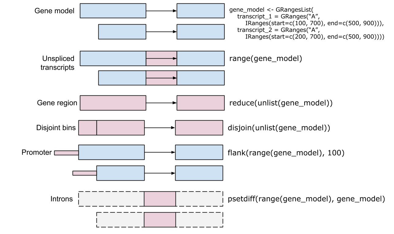
Ranges - IRanges - start() / end() / width() - Vector-like – length(), subset, etc. - ‘metadata’, mcols() - GRanges - ‘seqnames’ (chromosome), ‘strand’ - Seqinfo, including seqlevels and seqlengths
Intra-range methods - Independent of other ranges in the same object - GRanges variants strand-aware - shift(), narrow(), flank(), promoters(), resize(), restrict(), trim() - See ?"intra-range-methods"
Inter-range methods - Depends on other ranges in the same object - range(), reduce(), gaps(), disjoin() - coverage() (!) - see ?"inter-range-methods"
Between-range methods - Functions of two (or more) range objects - findOverlaps(), countOverlaps(), …, %over%, %within%, %outside%; union(), intersect(), setdiff(), punion(), pintersect(), psetdiff()
IRangesList, GRangesList - List: all elements of the same type - Many *List-aware methods, but a common ‘trick’: apply a vectorized function to the unlisted representaion, then re-list
grl <- GRangesList(...)
orig_gr <- unlist(grl)
transformed_gr <- FUN(orig)
transformed_grl <- relist(transformed_gr, grl)How to use high-throughput sequence data types in Bioconductor
The following sections briefly summarize some of the most important file types in high-throughput sequence analysis. Briefly review these, or those that are most relevant to your research, before starting on the section Data Representation in R / Bioconductor
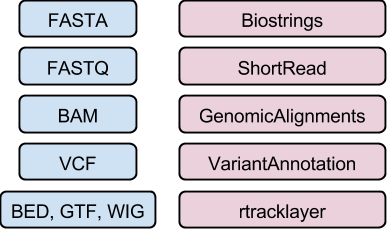
DNA / amino acid sequences: FASTA files
Input & manipulation: Biostrings
>NM_078863_up_2000_chr2L_16764737_f chr2L:16764737-16766736
gttggtggcccaccagtgccaaaatacacaagaagaagaaacagcatctt
gacactaaaatgcaaaaattgctttgcgtcaatgactcaaaacgaaaatg
...
atgggtatcaagttgccccgtataaaaggcaagtttaccggttgcacggt
>NM_001201794_up_2000_chr2L_8382455_f chr2L:8382455-8384454
ttatttatgtaggcgcccgttcccgcagccaaagcactcagaattccggg
cgtgtagcgcaacgaccatctacaaggcaatattttgatcgcttgttagg
...Reads: FASTQ files
Input & manipulation: ShortRead readFastq(), FastqStreamer(), FastqSampler()
@ERR127302.1703 HWI-EAS350_0441:1:1:1460:19184#0/1
CCTGAGTGAAGCTGATCTTGATCTACGAAGAGAGATAGATCTTGATCGTCGAGGAGATGCTGACCTTGACCT
+
HHGHHGHHHHHHHHDGG<GDGGE@GDGGD<?B8??ADAD<BE@EE8EGDGA3CB85*,77@>>CE?=896=:
@ERR127302.1704 HWI-EAS350_0441:1:1:1460:16861#0/1
GCGGTATGCTGGAAGGTGCTCGAATGGAGAGCGCCAGCGCCCCGGCGCTGAGCCGCAGCCTCAGGTCCGCCC
+
DE?DD>ED4>EEE>DE8EEEDE8B?EB<@3;BA79?,881B?@73;1?########################
- Quality scores: ‘phred-like’, encoded. See wikipedia
Aligned reads: BAM files (e.g., ERR127306_chr14.bam)
Input & manipulation: ‘low-level’ Rsamtools, scanBam(), BamFile(); ‘high-level’ GenomicAlignments
Header
@HD VN:1.0 SO:coordinate @SQ SN:chr1 LN:249250621 @SQ SN:chr10 LN:135534747 @SQ SN:chr11 LN:135006516 ... @SQ SN:chrY LN:59373566 @PG ID:TopHat VN:2.0.8b CL:/home/hpages/tophat-2.0.8b.Linux_x86_64/tophat --mate-inner-dist 150 --solexa-quals --max-multihits 5 --no-discordant --no-mixed --coverage-search --microexon-search --library-type fr-unstranded --num-threads 2 --output-dir tophat2_out/ERR127306 /home/hpages/bowtie2-2.1.0/indexes/hg19 fastq/ERR127306_1.fastq fastq/ERR127306_2.fastqAlignments: ID, flag, alignment and mate
ERR127306.7941162 403 chr14 19653689 3 72M = 19652348 -1413 ... ERR127306.22648137 145 chr14 19653692 1 72M = 19650044 -3720 ... ERR127306.933914 339 chr14 19653707 1 66M120N6M = 19653686 -213 ... ERR127306.11052450 83 chr14 19653707 3 66M120N6M = 19652348 -1551 ... ERR127306.24611331 147 chr14 19653708 1 65M120N7M = 19653675 -225 ... ERR127306.2698854 419 chr14 19653717 0 56M120N16M = 19653935 290 ... ERR127306.2698854 163 chr14 19653717 0 56M120N16M = 19653935 2019 ...Alignments: sequence and quality
... GAATTGATCAGTCTCATCTGAGAGTAACTTTGTACCCATCACTGATTCCTTCTGAGACTGCCTCCACTTCCC *'%%%%%#&&%''#'&%%%)&&%%$%%'%%'&*****$))$)'')'%)))&)%%%%$'%%%%&"))'')%)) ... TTGATCAGTCTCATCTGAGAGTAACTTTGTACCCATCACTGATTCCTTCTGAGACTGCCTCCACTTCCCCAG '**)****)*'*&*********('&)****&***(**')))())%)))&)))*')&***********)**** ... TGAGAGTAACTTTGTACCCATCACTGATTCCTTCTGAGACTGCCTCCACTTCCCCAGCAGCCTCTGGTTTCT '******&%)&)))&")')'')'*((******&)&'')'))$))'')&))$)**&&**************** ... TGAGAGTAACTTTGTACCCATCACTGATTCCTTCTGAGACTGCCTCCACTTCCCCAGCAGCCTCTGGTTTCT ##&&(#')$')'%&&#)%$#$%"%###&!%))'%%''%'))&))#)&%((%())))%)%)))%********* ... GAGAGTAACTTTGTACCCATCACTGATTCCTTCTGAGACTGCCTCCACTTCCCCAGCAGCCTCTGGTTTCTT )&$'$'$%!&&%&&#!'%'))%''&%'&))))''$""'%'%&%'#'%'"!'')#&)))))%$)%)&'"'))) ... TTTGTACCCATCACTGATTCCTTCTGAGACTGCCTCCACTTCCCCAGCAGCCTCTGGTTTCTTCATGTGGCT ++++++++++++++++++++++++++++++++++++++*++++++**++++**+**''**+*+*'*)))*)# ... TTTGTACCCATCACTGATTCCTTCTGAGACTGCCTCCACTTCCCCAGCAGCCTCTGGTTTCTTCATGTGGCT ++++++++++++++++++++++++++++++++++++++*++++++**++++**+**''**+*+*'*)))*)#Alignments: Tags
... AS:i:0 XN:i:0 XM:i:0 XO:i:0 XG:i:0 NM:i:0 MD:Z:72 YT:Z:UU NH:i:2 CC:Z:chr22 CP:i:16189276 HI:i:0 ... AS:i:0 XN:i:0 XM:i:0 XO:i:0 XG:i:0 NM:i:0 MD:Z:72 YT:Z:UU NH:i:3 CC:Z:= CP:i:19921600 HI:i:0 ... AS:i:0 XN:i:0 XM:i:0 XO:i:0 XG:i:0 NM:i:4 MD:Z:72 YT:Z:UU XS:A:+ NH:i:3 CC:Z:= CP:i:19921465 HI:i:0 ... AS:i:0 XN:i:0 XM:i:0 XO:i:0 XG:i:0 NM:i:4 MD:Z:72 YT:Z:UU XS:A:+ NH:i:2 CC:Z:chr22 CP:i:16189138 HI:i:0 ... AS:i:0 XN:i:0 XM:i:0 XO:i:0 XG:i:0 NM:i:5 MD:Z:72 YT:Z:UU XS:A:+ NH:i:3 CC:Z:= CP:i:19921464 HI:i:0 ... AS:i:0 XM:i:0 XO:i:0 XG:i:0 MD:Z:72 NM:i:0 XS:A:+ NH:i:5 CC:Z:= CP:i:19653717 HI:i:0 ... AS:i:0 XM:i:0 XO:i:0 XG:i:0 MD:Z:72 NM:i:0 XS:A:+ NH:i:5 CC:Z:= CP:i:19921455 HI:i:1
Called variants: VCF files
Input and manipulation: VariantAnnotation readVcf(), readInfo(), readGeno() selectively with ScanVcfParam().
Header
##fileformat=VCFv4.2 ##fileDate=20090805 ##source=myImputationProgramV3.1 ##reference=file:///seq/references/1000GenomesPilot-NCBI36.fasta ##contig=<ID=20,length=62435964,assembly=B36,md5=f126cdf8a6e0c7f379d618ff66beb2da,species="Homo sapiens",taxonomy=x> ##phasing=partial ##INFO=<ID=DP,Number=1,Type=Integer,Description="Total Depth"> ##INFO=<ID=AF,Number=A,Type=Float,Description="Allele Frequency"> ... ##FILTER=<ID=q10,Description="Quality below 10"> ##FILTER=<ID=s50,Description="Less than 50% of samples have data"> ... ##FORMAT=<ID=GT,Number=1,Type=String,Description="Genotype"> ##FORMAT=<ID=GQ,Number=1,Type=Integer,Description="Genotype Quality">Location
#CHROM POS ID REF ALT QUAL FILTER ... 20 14370 rs6054257 G A 29 PASS ... 20 17330 . T A 3 q10 ... 20 1110696 rs6040355 A G,T 67 PASS ... 20 1230237 . T . 47 PASS ... 20 1234567 microsat1 GTC G,GTCT 50 PASS ...Variant INFO
#CHROM POS ... INFO ... 20 14370 ... NS=3;DP=14;AF=0.5;DB;H2 ... 20 17330 ... NS=3;DP=11;AF=0.017 ... 20 1110696 ... NS=2;DP=10;AF=0.333,0.667;AA=T;DB ... 20 1230237 ... NS=3;DP=13;AA=T ... 20 1234567 ... NS=3;DP=9;AA=G ...Genotype FORMAT and samples
... POS ... FORMAT NA00001 NA00002 NA00003 ... 14370 ... GT:GQ:DP:HQ 0|0:48:1:51,51 1|0:48:8:51,51 1/1:43:5:.,. ... 17330 ... GT:GQ:DP:HQ 0|0:49:3:58,50 0|1:3:5:65,3 0/0:41:3 ... 1110696 ... GT:GQ:DP:HQ 1|2:21:6:23,27 2|1:2:0:18,2 2/2:35:4 ... 1230237 ... GT:GQ:DP:HQ 0|0:54:7:56,60 0|0:48:4:51,51 0/0:61:2 ... 1234567 ... GT:GQ:DP 0/1:35:4 0/2:17:2 1/1:40:3
Genome annotations: BED, WIG, GTF, etc. files
Input: rtracklayer import()
BED: range-based annotation (see http://genome.ucsc.edu/FAQ/FAQformat.html for definition of this and related formats)
WIG / bigWig: dense, continuous-valued data
GTF: gene model
Component coordinates
7 protein_coding gene 27221129 27224842 . - . ... ... 7 protein_coding transcript 27221134 27224835 . - . ... 7 protein_coding exon 27224055 27224835 . - . ... 7 protein_coding CDS 27224055 27224763 . - 0 ... 7 protein_coding start_codon 27224761 27224763 . - 0 ... 7 protein_coding exon 27221134 27222647 . - . ... 7 protein_coding CDS 27222418 27222647 . - 2 ... 7 protein_coding stop_codon 27222415 27222417 . - 0 ... 7 protein_coding UTR 27224764 27224835 . - . ... 7 protein_coding UTR 27221134 27222414 . - . ...Annotations
gene_id "ENSG00000005073"; gene_name "HOXA11"; gene_source "ensembl_havana"; gene_biotype "protein_coding"; ... ... transcript_id "ENST00000006015"; transcript_name "HOXA11-001"; transcript_source "ensembl_havana"; tag "CCDS"; ccds_id "CCDS5411"; ... exon_number "1"; exon_id "ENSE00001147062"; ... exon_number "1"; protein_id "ENSP00000006015"; ... exon_number "1"; ... exon_number "2"; exon_id "ENSE00002099557"; ... exon_number "2"; protein_id "ENSP00000006015"; ... exon_number "2"; ... ...
Exercises: sequence data representation in R / Bioconductor
This section briefly illustrates how different high-throughput sequence data types are represented in R / Bioconductor. Select relevant data types for your area of interest, and work through the examples. Take time to consult help pages, understand the output of function calls, and the relationship between standard data formats (summarized in the previous section) and the corresponding R / Bioconductor representation.
Biostrings (DNA or amino acid sequences)
Classes
- XString, XStringSet, e.g., DNAString (genomes), DNAStringSet (reads)
Methods –
- Cheat sheat
- Manipulation, e.g.,
reverseComplement() - Summary, e.g.,
letterFrequency() - Matching, e.g.,
matchPDict(),matchPWM()
Related packages
Example
- Whole-genome sequences are distrubuted by ENSEMBL, NCBI, and others as FASTA files; model organism whole genome sequences are packaged into more user-friendly
BSgenomepackages. The following calculates GC content across chr14.
library("BSgenome.Hsapiens.UCSC.hg38")
chr14_range <- GRanges("chr14", IRanges(1, seqlengths(Hsapiens)["chr14"]))
chr14_dna <- getSeq(Hsapiens, chr14_range)
letterFrequency(chr14_dna, "GC", as.prob=TRUE) G|C
[1,] 0.336276Exercises
Setup
- Mouse CDS sequence, from Ensembl: https://useast.ensembl.org/info/data/ftp/index.html
url <- "ftp://ftp.ensembl.org/pub/release-92/fasta/mus_musculus/cds/Mus_musculus.GRCm38.cds.all.fa.gz"
fl <- BiocFileCache::bfcrpath(rnames = url)
cds <- rtracklayer::import(fl, "fasta")- For simplicity, clean up the data to remove cds with width not a multiple of three. Remove cds that don’t start with a start codon
ATGor end with a stop codonc("TAA", "TAG", "TGA")
pred1 <- width(cds) %% 3 == 0
table(pred1)pred1
FALSE TRUE
7219 58251 pred2 <- narrow(cds, 1, 3) == "ATG"
stops <- c("TAA", "TAG", "TGA")
pred3 <- narrow(cds, width(cds) - 2, width(cds)) %in% stops
table(pred1 & pred2 & pred3)
FALSE TRUE
16808 48662 cds <- cds[ pred1 & pred2 & pred3 ]- What does the distribution of widths of the cds look like? Which cds has maximum width?
hist(log10(width(cds)))
cds[ which.max(width(cds)) ]DNAStringSet object of length 1:
width seq names
[1] 105642 ATGACTACTCAAGCACCGATGTT...TATTAATATCCGTTCTATGTAA ENSMUST0000009998...names(cds)[ which.max(width(cds)) ][1] "ENSMUST00000099981.8 cds chromosome:GRCm38:2:76703980:76982455:-1 gene:ENSMUSG00000051747.14 gene_biotype:protein_coding transcript_biotype:protein_coding gene_symbol:Ttn description:titin [Source:MGI Symbol;Acc:MGI:98864]"- Use the
letterFrequencyfunction to calculate the GC content of each cds; visualize the distribution of GC content.
gc <- letterFrequency(cds, "GC", as.prob=TRUE)
head(gc) G|C
[1,] 0.5026624
[2,] 0.5026624
[3,] 0.5026624
[4,] 0.4879075
[5,] 0.5066079
[6,] 0.5714286hist(gc)
plot( log10(width(cds)), gc, pch=".")
- Summarize codon usage in each CDS. Which codons are used most frequently over all CDS?
AMINO_ACID_CODE A R N D C Q E G H I L K M
"Ala" "Arg" "Asn" "Asp" "Cys" "Gln" "Glu" "Gly" "His" "Ile" "Leu" "Lys" "Met"
F P S T W Y V U O B J Z X
"Phe" "Pro" "Ser" "Thr" "Trp" "Tyr" "Val" "Sec" "Pyl" "Asx" "Xle" "Glx" "Xaa" aa <- translate(cds)
codon_use <- letterFrequency(aa, names(AMINO_ACID_CODE))
head(codon_use) A R N D C Q E G H I L K M F P S T W Y V U O B J Z X
[1,] 17 12 10 7 11 12 11 14 5 20 47 12 6 23 17 24 19 3 11 30 0 0 0 0 0 0
[2,] 17 12 10 7 11 12 11 14 5 20 47 12 6 23 17 24 19 3 11 30 0 0 0 0 0 0
[3,] 17 12 10 7 11 12 11 14 5 20 47 12 6 23 17 24 19 3 11 30 0 0 0 0 0 0
[4,] 25 11 8 6 5 5 7 11 10 34 40 11 10 20 14 36 26 2 11 23 0 0 0 0 0 0
[5,] 36 25 22 26 15 38 30 40 20 27 63 32 11 24 40 86 59 11 34 40 0 0 0 0 0 0
[6,] 0 0 0 0 14 10 5 0 0 0 2 8 1 1 29 3 1 0 0 2 0 0 0 0 0 0- (Advanced) –
DNAStringSetinherits fromVectorandAnnotated, which means that each element (sequence) can have additional information, for instance we can associate GC content with each sequence
mcols(cds) <- DataFrame(GC = gc[,"G|C"])
mcols(cds, use.names = FALSE)DataFrame with 48662 rows and 1 column
GC
<numeric>
1 0.502662
2 0.502662
3 0.502662
4 0.487907
5 0.506608
... ...
48658 0.627869
48659 0.625755
48660 0.659102
48661 0.649718
48662 0.596270mcols(cds[1:3], use.names = FALSE)DataFrame with 3 rows and 1 column
GC
<numeric>
1 0.502662
2 0.502662
3 0.502662SummarizedExperiment
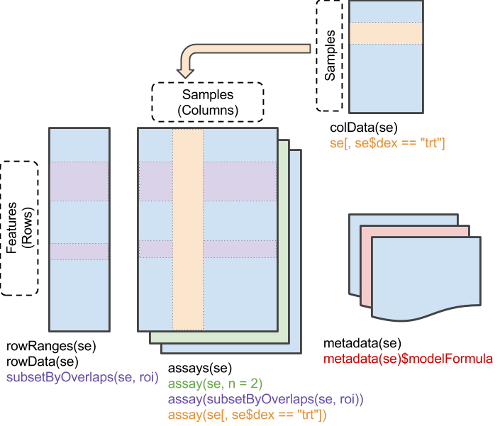
Motivation: reproducible & interoperable
Matrix of feature x sample measurements,
assays()Addition description about samples,
colData()- Covariates, e.g., age, gender
- Experimental design, e.g., treatment group
Additional information about features,
rowData()- Gene names, width, GC content, …
- Genomic ranges(!)
- Derived values, E.g., log-fold change between treatments, P-value, …
Information about the experiment as a whole –
metadata()
Example 1: Bulk RNA-seq airway data
- Attach the airway library and data set
library("airway")
data("airway")
airwayclass: RangedSummarizedExperiment
dim: 63677 8
metadata(1): ''
assays(1): counts
rownames(63677): ENSG00000000003 ENSG00000000005 ... ENSG00000273492
ENSG00000273493
rowData names(10): gene_id gene_name ... seq_coord_system symbol
colnames(8): SRR1039508 SRR1039509 ... SRR1039520 SRR1039521
colData names(9): SampleName cell ... Sample BioSample- Explore the phenotypic data describing samples. Subset to include just the
untrtsamples.
colData(airway)DataFrame with 8 rows and 9 columns
SampleName cell dex albut Run avgLength
<factor> <factor> <factor> <factor> <factor> <integer>
SRR1039508 GSM1275862 N61311 untrt untrt SRR1039508 126
SRR1039509 GSM1275863 N61311 trt untrt SRR1039509 126
SRR1039512 GSM1275866 N052611 untrt untrt SRR1039512 126
SRR1039513 GSM1275867 N052611 trt untrt SRR1039513 87
SRR1039516 GSM1275870 N080611 untrt untrt SRR1039516 120
SRR1039517 GSM1275871 N080611 trt untrt SRR1039517 126
SRR1039520 GSM1275874 N061011 untrt untrt SRR1039520 101
SRR1039521 GSM1275875 N061011 trt untrt SRR1039521 98
Experiment Sample BioSample
<factor> <factor> <factor>
SRR1039508 SRX384345 SRS508568 SAMN02422669
SRR1039509 SRX384346 SRS508567 SAMN02422675
SRR1039512 SRX384349 SRS508571 SAMN02422678
SRR1039513 SRX384350 SRS508572 SAMN02422670
SRR1039516 SRX384353 SRS508575 SAMN02422682
SRR1039517 SRX384354 SRS508576 SAMN02422673
SRR1039520 SRX384357 SRS508579 SAMN02422683
SRR1039521 SRX384358 SRS508580 SAMN02422677airway[ , airway$dex == "untrt"]class: RangedSummarizedExperiment
dim: 63677 4
metadata(1): ''
assays(1): counts
rownames(63677): ENSG00000000003 ENSG00000000005 ... ENSG00000273492
ENSG00000273493
rowData names(10): gene_id gene_name ... seq_coord_system symbol
colnames(4): SRR1039508 SRR1039512 SRR1039516 SRR1039520
colData names(9): SampleName cell ... Sample BioSample- Calculate library size as the column sums of the assays. Reflect on the relationship between library size and cell / dex column variables and consequences for differential expression analysis.
colSums(assay(airway))SRR1039508 SRR1039509 SRR1039512 SRR1039513 SRR1039516 SRR1039517 SRR1039520
20637971 18809481 25348649 15163415 24448408 30818215 19126151
SRR1039521
21164133 Example 2 (advanced): single-cell RNA-seq.
- Retrieve mouse embryo data derived from La Manno A et al., 2016, Molecular diversity of midbrain development in mouse, human, and stem cells; Cell 167(2), 566-580.
sce <- scRNAseq::LaMannoBrainData("mouse-embryo")Exercises
- What is the frequency of 0 counts in the single cell assay data?
- What is the distribution of library sizes in the single cell assay data?
- Create a random sample of 100 cells and visualize the relationship between samples using
dist()andcmdscale(). - can you identify what column of
colData()is responsible for any pattern you see? - In exploring the covariates, are the possible problems with confounding?
GenomicRanges
Example
library("GenomicRanges")
gr <- GRanges(c("chr1:10-14:+", "chr1:20-24:+", "chr1:22-26:+"))
shift(gr, 1) # 1-based coordinates!GRanges object with 3 ranges and 0 metadata columns:
seqnames ranges strand
<Rle> <IRanges> <Rle>
[1] chr1 11-15 +
[2] chr1 21-25 +
[3] chr1 23-27 +
-------
seqinfo: 1 sequence from an unspecified genome; no seqlengthsrange(gr) # intra-rangeGRanges object with 1 range and 0 metadata columns:
seqnames ranges strand
<Rle> <IRanges> <Rle>
[1] chr1 10-26 +
-------
seqinfo: 1 sequence from an unspecified genome; no seqlengthsreduce(gr) # inter-rangeGRanges object with 2 ranges and 0 metadata columns:
seqnames ranges strand
<Rle> <IRanges> <Rle>
[1] chr1 10-14 +
[2] chr1 20-26 +
-------
seqinfo: 1 sequence from an unspecified genome; no seqlengthscoverage(gr)RleList of length 1
$chr1
integer-Rle of length 26 with 6 runs
Lengths: 9 5 5 2 3 2
Values : 0 1 0 1 2 1setdiff(range(gr), gr) # 'introns'GRanges object with 1 range and 0 metadata columns:
seqnames ranges strand
<Rle> <IRanges> <Rle>
[1] chr1 15-19 +
-------
seqinfo: 1 sequence from an unspecified genome; no seqlengthsExercises
- Which of my SNPs overlap genes?
genes <- GRanges(c("chr1:30-40:+", "chr1:60-70:-"))
snps <- GRanges(c("chr1:35", "chr1:60", "chr1:45"))
countOverlaps(snps, genes) > 0[1] TRUE TRUE FALSE- Which gene is ‘nearest’ my regulatory region? Which gene does my regulatory region precede (i.e., upstream of)
reg <- GRanges(c("chr1:50-55", "chr1:75-80"))
nearest(reg, genes)[1] 2 2precede(reg, genes)[1] NA 2- What range do short reads cover? depth of coverage?
reads <- GRanges(c("chr1:10-19", "chr1:15-24", "chr1:30-41"))
coverage(reads, width = 100)RleList of length 1
$chr1
integer-Rle of length 100 with 7 runs
Lengths: 9 5 5 5 5 12 59
Values : 0 1 2 1 0 1 0as(coverage(reads, width = 100), "GRanges")GRanges object with 7 ranges and 1 metadata column:
seqnames ranges strand | score
<Rle> <IRanges> <Rle> | <integer>
[1] chr1 1-9 * | 0
[2] chr1 10-14 * | 1
[3] chr1 15-19 * | 2
[4] chr1 20-24 * | 1
[5] chr1 25-29 * | 0
[6] chr1 30-41 * | 1
[7] chr1 42-100 * | 0
-------
seqinfo: 1 sequence from an unspecified genomeReference
- Lawrence M, Huber W, Pagès H, Aboyoun P, Carlson M, et al. (2013) Software for Computing and Annotating Genomic Ranges. PLoS Comput Biol 9(8): e1003118. doi:10.1371/journal.pcbi.1003118
GenomicAlignments (Aligned reads)
Classes – GenomicRanges-like behaivor
- GAlignments, GAlignmentPairs, GAlignmentsList
Methods
readGAlignments(),readGAlignmentsList()- Easy to restrict input, iterate in chunks
summarizeOverlaps()
Exercises
- Find reads supporting the junction identified above, at position 19653707 + 66M = 19653773 of chromosome 14
library("GenomicRanges")
library("GenomicAlignments")
library("Rsamtools")
## our 'region of interest'
roi <- GRanges("chr14", IRanges(19653773, width=1))
## sample data
library("RNAseqData.HNRNPC.bam.chr14")
bf <- BamFile(RNAseqData.HNRNPC.bam.chr14_BAMFILES[[1]], asMates=TRUE)
## alignments, junctions, overlapping our roi
paln <- readGAlignmentsList(bf)
j <- summarizeJunctions(paln, with.revmap=TRUE)
j_overlap <- j[j %over% roi]
## supporting reads
paln[j_overlap$revmap[[1]]]GAlignmentsList object of length 8:
[[1]]
GAlignments object with 2 alignments and 0 metadata columns:
seqnames strand cigar qwidth start end width
<Rle> <Rle> <character> <integer> <integer> <integer> <integer>
[1] chr14 - 66M120N6M 72 19653707 19653898 192
[2] chr14 + 7M1270N65M 72 19652348 19653689 1342
njunc
<integer>
[1] 1
[2] 1
-------
seqinfo: 93 sequences from an unspecified genome
[[2]]
GAlignments object with 2 alignments and 0 metadata columns:
seqnames strand cigar qwidth start end width
<Rle> <Rle> <character> <integer> <integer> <integer> <integer>
[1] chr14 - 66M120N6M 72 19653707 19653898 192
[2] chr14 + 72M 72 19653686 19653757 72
njunc
<integer>
[1] 1
[2] 0
-------
seqinfo: 93 sequences from an unspecified genome
[[3]]
GAlignments object with 2 alignments and 0 metadata columns:
seqnames strand cigar qwidth start end width
<Rle> <Rle> <character> <integer> <integer> <integer> <integer>
[1] chr14 + 72M 72 19653675 19653746 72
[2] chr14 - 65M120N7M 72 19653708 19653899 192
njunc
<integer>
[1] 0
[2] 1
-------
seqinfo: 93 sequences from an unspecified genome
...
<5 more elements>VariantAnnotation (Called variants)
Classes – GenomicRanges-like behavior
- VCF – ‘wide’
- VRanges – ‘tall’
Functions and methods
- I/O and filtering:
readVcf(),readGeno(),readInfo(),readGT(),writeVcf(),filterVcf() - Annotation:
locateVariants()(variants overlapping ranges),predictCoding(),summarizeVariants() - SNPs:
genotypeToSnpMatrix(),snpSummary()
Exerises
- Read variants from a VCF file, and annotate with respect to a known gene model
## input variants
library("VariantAnnotation")
fl <- system.file("extdata", "chr22.vcf.gz", package="VariantAnnotation")
vcf <- readVcf(fl, "hg19")
seqlevels(vcf) <- "chr22"
## known gene model
library("TxDb.Hsapiens.UCSC.hg19.knownGene")
coding <- locateVariants(
rowRanges(vcf),
TxDb.Hsapiens.UCSC.hg19.knownGene,
CodingVariants()
)Warning in valid.GenomicRanges.seqinfo(x, suggest.trim = TRUE): GRanges object contains 11135 out-of-bound ranges located on sequences
368369, 364612, 364613, 364614, 364616, 364617, 364628, 368375, 368376,
368377, 364634, 364629, 364632, 364636, 364637, 364638, 364639, 364640,
364642, 364643, 364645, 364646, 368396, 368397, 368400, 368402, 368406,
368411, 368405, 368401, 368403, 368404, 368425, 368443, 368445, 368447,
368453, 364662, 364663, 364655, 364656, 364657, 364658, 364660, 368456,
368462, 368470, 368471, 368472, 368474, 368475, 368476, 368477, 368478,
368481, 368486, 368491, 368490, 368494, 368495, 368488, 368483, 368473,
368469, 368485, 364666, 364667, 364668, 364669, 364670, 364671, 368522,
364672, 364673, 364674, 364676, 364678, 364681, 368533, 368541, 368555,
368553, 368554, 368556, 368573, and 368574. Note that ranges located on a
sequence whose length is unknown (NA) or on a circular sequence are not
considered out-of-bound (use seqlengths() and isCircular() to get the lengths
and circularity flags of the underlying sequences). You can use trim() to
trim these ranges. See ?`trim,GenomicRanges-method` for more information.head(coding)GRanges object with 6 ranges and 9 metadata columns:
seqnames ranges strand | LOCATION LOCSTART LOCEND
<Rle> <IRanges> <Rle> | <factor> <integer> <integer>
rs114335781 chr22 50301422 - | coding 939 939
rs114335781 chr22 50301422 - | coding 145 145
rs114335781 chr22 50301422 - | coding 470 470
rs8135963 chr22 50301476 - | coding 885 885
rs8135963 chr22 50301476 - | coding 91 91
rs8135963 chr22 50301476 - | coding 416 416
QUERYID TXID CDSID GENEID PRECEDEID
<integer> <character> <IntegerList> <character> <CharacterList>
rs114335781 24 368369 268191,268190 79087
rs114335781 24 368370 268191,268190 79087
rs114335781 24 368371 268191,268190 79087
rs8135963 25 368369 268191,268190 79087
rs8135963 25 368370 268191,268190 79087
rs8135963 25 368371 268191,268190 79087
FOLLOWID
<CharacterList>
rs114335781
rs114335781
rs114335781
rs8135963
rs8135963
rs8135963
-------
seqinfo: 1 sequence from an unspecified genome; no seqlengthsRelated packages
- ensemblVEP
- Forward variants to Ensembl Variant Effect Predictor
- VariantTools, h5vc
- Call variants
Reference
- Obenchain, V, Lawrence, M, Carey, V, Gogarten, S, Shannon, P, and Morgan, M. VariantAnnotation: a Bioconductor package for exploration and annotation of genetic variants. Bioinformatics, first published online March 28, 2014 doi:10.1093/bioinformatics/btu168
rtracklayer (Genome annotations)
- Import BED, GTF, WIG, etc
- Export GRanges to BED, GTF, WIG, …
- Access UCSC genome browser
Extended exercises
Summarize overlaps
The goal is to count the number of reads overlapping exons grouped into genes. This type of count data is the basic input for RNASeq differential expression analysis, e.g., through DESeq2 and edgeR.
- Identify the regions of interest. We use a ‘TxDb’ package with gene models already defined; the genome (hg19) is determined by the genome used for read alignment in the sample BAM files.
library("TxDb.Hsapiens.UCSC.hg19.knownGene")
exByGn <- exonsBy(TxDb.Hsapiens.UCSC.hg19.knownGene, "gene")
## only chromosome 14
seqlevels(exByGn, pruning.mode="coarse") = "chr14"- Identify the sample BAM files.
library("RNAseqData.HNRNPC.bam.chr14")
length(RNAseqData.HNRNPC.bam.chr14_BAMFILES)[1] 8- Summarize overlaps, optionally in parallel
## next 2 lines optional; non-Windows
library("BiocParallel")
register(MulticoreParam(workers=parallel::detectCores()))
olaps <- summarizeOverlaps(exByGn, RNAseqData.HNRNPC.bam.chr14_BAMFILES)- Explore our handiwork, e.g., library sizes (column sums), relationship between gene length and number of mapped reads, etc.
olapsclass: RangedSummarizedExperiment
dim: 946 8
metadata(0):
assays(1): counts
rownames(946): 10001 100113389 ... 9950 9985
rowData names(0):
colnames(8): ERR127306 ERR127307 ... ERR127304 ERR127305
colData names(0):head(assay(olaps)) ERR127306 ERR127307 ERR127308 ERR127309 ERR127302 ERR127303 ERR127304
10001 104 142 113 126 155 172 185
100113389 0 0 0 0 0 0 0
100113391 0 0 0 0 0 0 0
100124539 0 0 0 0 0 0 0
100126297 0 0 0 0 0 0 0
100126308 0 0 0 0 0 0 0
ERR127305
10001 151
100113389 0
100113391 0
100124539 0
100126297 0
100126308 0colSums(assay(olaps)) # library sizesERR127306 ERR127307 ERR127308 ERR127309 ERR127302 ERR127303 ERR127304 ERR127305
357059 391468 389764 347592 330840 348481 350115 347293 plot(x = log10(sum(width(olaps))),
y = log10(1 + rowMeans(assay(olaps))), asp = 1, pch = 16)
- As an advanced exercise, investigate the relationship between GC content and read count
library("BSgenome.Hsapiens.UCSC.hg19")
sequences <- getSeq(BSgenome.Hsapiens.UCSC.hg19, rowRanges(olaps))
gcPerExon <- letterFrequency(unlist(sequences), "GC")
gc <- relist(as.vector(gcPerExon), sequences)
gc_percent <- sum(gc) / sum(width(olaps))
plot(gc_percent, log10(1 + rowMeans(assay(olaps))), pch = 16)
End matter
Session Info
sessionInfo()R version 4.6.0 (2026-04-24)
Platform: aarch64-apple-darwin23
Running under: macOS Tahoe 26.4.1
Matrix products: default
BLAS: /Library/Frameworks/R.framework/Versions/4.6/Resources/lib/libRblas.0.dylib
LAPACK: /Library/Frameworks/R.framework/Versions/4.6/Resources/lib/libRlapack.dylib; LAPACK version 3.12.1
locale:
[1] en_US.UTF-8/en_US.UTF-8/en_US.UTF-8/C/en_US.UTF-8/en_US.UTF-8
time zone: Europe/Berlin
tzcode source: internal
attached base packages:
[1] stats4 stats graphics grDevices utils datasets methods
[8] base
other attached packages:
[1] BSgenome.Hsapiens.UCSC.hg19_1.4.3
[2] BiocParallel_1.46.0
[3] TxDb.Hsapiens.UCSC.hg19.knownGene_3.22.1
[4] GenomicFeatures_1.64.0
[5] AnnotationDbi_1.74.0
[6] VariantAnnotation_1.58.0
[7] RNAseqData.HNRNPC.bam.chr14_0.50.0
[8] GenomicAlignments_1.48.0
[9] Rsamtools_2.28.0
[10] airway_1.32.0
[11] SummarizedExperiment_1.42.0
[12] Biobase_2.72.0
[13] MatrixGenerics_1.24.0
[14] matrixStats_1.5.0
[15] BSgenome.Hsapiens.UCSC.hg38_1.4.5
[16] BSgenome_1.80.0
[17] rtracklayer_1.72.0
[18] BiocIO_1.22.0
[19] GenomeInfoDb_1.48.0
[20] pwalign_1.8.0
[21] GenomicRanges_1.64.0
[22] Biostrings_2.80.0
[23] Seqinfo_1.2.0
[24] XVector_0.52.0
[25] IRanges_2.46.0
[26] S4Vectors_0.50.0
[27] BiocGenerics_0.58.0
[28] generics_0.1.4
[29] BiocStyle_2.40.0
loaded via a namespace (and not attached):
[1] DBI_1.3.0 bitops_1.0-9
[3] httr2_1.2.2 rlang_1.2.0
[5] magrittr_2.0.5 gypsum_1.8.0
[7] compiler_4.6.0 RSQLite_2.4.6
[9] png_0.1-9 vctrs_0.7.3
[11] ProtGenerics_1.44.0 pkgconfig_2.0.3
[13] crayon_1.5.3 fastmap_1.2.0
[15] dbplyr_2.5.2 rmarkdown_2.31
[17] UCSC.utils_1.8.0 scRNAseq_2.26.0
[19] purrr_1.2.2 bit_4.6.0
[21] xfun_0.57 cachem_1.1.0
[23] cigarillo_1.2.0 jsonlite_2.0.0
[25] blob_1.3.0 rhdf5filters_1.24.0
[27] DelayedArray_0.38.1 Rhdf5lib_2.0.0
[29] parallel_4.6.0 R6_2.6.1
[31] Rcpp_1.1.1-1.1 knitr_1.51
[33] Matrix_1.7-5 tidyselect_1.2.1
[35] rstudioapi_0.18.0 abind_1.4-8
[37] yaml_2.3.12 codetools_0.2-20
[39] curl_7.1.0 lattice_0.22-9
[41] alabaster.sce_1.12.0 tibble_3.3.1
[43] withr_3.0.2 KEGGREST_1.52.0
[45] evaluate_1.0.5 BiocFileCache_3.2.0
[47] alabaster.schemas_1.12.0 ExperimentHub_3.2.0
[49] pillar_1.11.1 BiocManager_1.30.27
[51] filelock_1.0.3 RCurl_1.98-1.18
[53] BiocVersion_3.23.1 ensembldb_2.36.0
[55] alabaster.base_1.13.0 alabaster.ranges_1.12.0
[57] glue_1.8.1 alabaster.matrix_1.12.0
[59] lazyeval_0.2.3 tools_4.6.0
[61] AnnotationHub_4.2.0 XML_3.99-0.23
[63] rhdf5_2.56.0 grid_4.6.0
[65] SingleCellExperiment_1.34.0 HDF5Array_1.40.0
[67] restfulr_0.0.16 cli_3.6.6
[69] rappdirs_0.3.4 S4Arrays_1.12.0
[71] dplyr_1.2.1 AnnotationFilter_1.36.0
[73] alabaster.se_1.12.0 digest_0.6.39
[75] SparseArray_1.12.2 rjson_0.2.23
[77] htmlwidgets_1.6.4 memoise_2.0.1
[79] htmltools_0.5.9 lifecycle_1.0.5
[81] h5mread_1.4.0 httr_1.4.8
[83] bit64_4.8.0 Acknowledgements
Research reported in this tutorial was supported by the National Human Genome Research Institute and the National Cancer Institute of the National Institutes of Health under award numbers U24HG004059 (Bioconductor), U24HG010263 (AnVIL) and U24CA180996 (ITCR).